Practice: Chp. 11#

source("iplot.R")
suppressPackageStartupMessages(library(rethinking))

11E1. If an event has probability 0.35, what are the log-odds of this event?

Answer. The odds are $0.35 / (1 - 0.35) = 0.35/0.65$ or about a half. The odds (Odds) in favor of the event are about one to two. On the log2 scale we should expect the log-odds to be about negative one:

\[ log2\left(\frac{p}{1-p}\right) = log2(0.35 / (1 - 0.35)) = -0.893 \]

For a logarithmic base of e contract the log scale by log(2) or about 0.7:

\[ log\left(\frac{p}{1-p}\right) = log(0.35 / (1 - 0.35)) = -0.619 \]

11E2. If an event has log-odds 3.2, what is the probability of the event?

Answer. Expect a log2-odds of about 3.2/0.7 or around 4.6. That is, the odds in favor of the event should be about 2**4.6 to one, perhaps around 25:1.

\[ \frac{1}{1+e^{-x}} = \frac{1}{1+e^{-3.2}} = 0.961 \]

11E3. Suppose that a coefficient in a logistic regression has value 1.7. What does this imply about the proportional change in odds of the outcome?

Answer. The ‘proportional odds’ is about five:

\[ q = e^{\beta} = e^{1.7} = 5.47 \]

The ‘proportional odds’ is the change in odds for a unit increase in the predictor variable. So when the predictor variable increases by one, we can expect the odds $p/(1-p)$ to increase by about a factor of five.

11E4. Why do Poisson regressions sometimes require the use of an offset? Provide an example.

Answer. We use an offset in a Poisson regression (see section 11.2.3) when we have counts that were collected at varying densities. For example, counts collected over varying:

Lengths of observation
Area of sampling
Intensity of sampling

The offset lets us include all the data in the same model while still accounting for the differences in measurement.

A specific example would be collecting the number of visitors to a restaurant. Some counts may be collected on a daily basis, and others on a weekly basis.

11M1. As explained in the chapter, binomial data can be organized in aggregated and disaggregated forms, without any impact on inference. But the likelihood of the data does change when the data are converted between the two formats. Can you explain why?

Answer. The likelihood changes when you move from the disaggregated to aggregated format because now there is no longer exactly one trial associated with every event.

11M2. If a coefficient in a Poisson regression has value 1.7, what does this imply about the change in outcome?

Answer. Assuming the Poisson regression uses a log link, for a unit increase in the predictor variable we should see an increase in the rate (or mean) $\lambda$ of about five:

\[ q = \frac{exp(\alpha + \beta (x + 1))}{exp(\alpha + \beta x)} = exp(\beta) = exp(1.7) \approx 5.47 \]

11M3. Explain why the logit link is appropriate for a binomial generalized linear model.

Answer. The binomial distribution takes a probability parameter (between zero and one) and the logit link constrains a parameter to this range.

11M4. Explain why the log link is appropriate for a Poisson generalized linear model.

Answer. The Poisson distribution takes a positive real-valued parameter and the log link constrains a parameter to this range.

11M5. What would it imply to use a logit link for the mean of a Poisson generalized linear model? Can you think of a real research problem for which this would make sense?

Answer. It would imply the mean $\lambda$ is between zero and one, rather than simply positive and real-valued. If the researcher knows the maximum number of times (e.g. one) an event can occur, it seems like it would be more appropriate to use the binomial distribution in many cases and infer p instead.

11M6. State the constraints for which the binomial and Poisson distributions have maximum entropy. Are the constraints different at all for binomial and Poisson? Why or why not?

Answer. The maximum entropy constraint for both these distributions is that the expected value is a constant. See Maximum entropy probability distribution.

These constraints are the same because the Poisson distribution is an approximation of the binomial when p is small and N is large. See Poisson approximation.

11M7. Use quap to construct a quadratic approximate posterior distribution for the chimpanzee model that includes a unique intercept for each actor, m11.4 (page 330). Compare the quadratic approximation to the posterior distribution produced instead from MCMC. Can you explain both the differences and the similarities between the approximate and the MCMC distributions? Relax the prior on the actor intercepts to Normal(0, 10). Re-estimate the posterior using both ulam and quap. Do the differences increase or decrease? Why?

Answer. The quadratic approximation assumes a symmetric Gaussian posterior, so it may produce posterior inferences that are more symmetric (unlike MCMC). In this case, the algorithms produce marginally different results.

When we move to the flat prior, quap struggles to produce a decent result because it is starting with a prior that is completely non-symmetric. It may pick either the left or the right peak of the prior to optimize from.

source('practice11/load-chimp-models.R')
flush.console()

m11.4_flat_prior <- ulam(
  alist(
    pulled_left ~ dbinom(1, p),
    logit(p) <- a[actor] + b[treatment],
    a[actor] ~ dnorm(0, 10),
    b[treatment] ~ dnorm(0, 0.5)
  ),
  data = dat_list, chains = 4, log_lik = TRUE
)

m11.4_quap_flat_prior <- quap(
  m11.4_flat_prior@formula,
  data = dat_list
)
flush.console()

iplot(function() {
  plot(compare(m11.4, m11.4_quap, m11.4_flat_prior, m11.4_quap_flat_prior))
}, ar=3)

SAMPLING FOR MODEL '82480dff1a626a42c2ca9de938d65b9d' NOW (CHAIN 1).
Chain 1: 
Chain 1: Gradient evaluation took 7e-05 seconds
Chain 1: 1000 transitions using 10 leapfrog steps per transition would take 0.7 seconds.
Chain 1: Adjust your expectations accordingly!
Chain 1: 
Chain 1: 
Chain 1: Iteration:   1 / 1000 [  0%]  (Warmup)
Chain 1: Iteration: 100 / 1000 [ 10%]  (Warmup)
Chain 1: Iteration: 200 / 1000 [ 20%]  (Warmup)
Chain 1: Iteration: 300 / 1000 [ 30%]  (Warmup)
Chain 1: Iteration: 400 / 1000 [ 40%]  (Warmup)
Chain 1: Iteration: 500 / 1000 [ 50%]  (Warmup)
Chain 1: Iteration: 501 / 1000 [ 50%]  (Sampling)
Chain 1: Iteration: 600 / 1000 [ 60%]  (Sampling)
Chain 1: Iteration: 700 / 1000 [ 70%]  (Sampling)
Chain 1: Iteration: 800 / 1000 [ 80%]  (Sampling)
Chain 1: Iteration: 900 / 1000 [ 90%]  (Sampling)
Chain 1: Iteration: 1000 / 1000 [100%]  (Sampling)
Chain 1: 
Chain 1:  Elapsed Time: 0.531393 seconds (Warm-up)
Chain 1:                0.462519 seconds (Sampling)
Chain 1:                0.993912 seconds (Total)
Chain 1: 

SAMPLING FOR MODEL '82480dff1a626a42c2ca9de938d65b9d' NOW (CHAIN 2).
Chain 2: 
Chain 2: Gradient evaluation took 6.1e-05 seconds
Chain 2: 1000 transitions using 10 leapfrog steps per transition would take 0.61 seconds.
Chain 2: Adjust your expectations accordingly!
Chain 2: 
Chain 2: 
Chain 2: Iteration:   1 / 1000 [  0%]  (Warmup)
Chain 2: Iteration: 100 / 1000 [ 10%]  (Warmup)
Chain 2: Iteration: 200 / 1000 [ 20%]  (Warmup)
Chain 2: Iteration: 300 / 1000 [ 30%]  (Warmup)
Chain 2: Iteration: 400 / 1000 [ 40%]  (Warmup)
Chain 2: Iteration: 500 / 1000 [ 50%]  (Warmup)
Chain 2: Iteration: 501 / 1000 [ 50%]  (Sampling)
Chain 2: Iteration: 600 / 1000 [ 60%]  (Sampling)
Chain 2: Iteration: 700 / 1000 [ 70%]  (Sampling)
Chain 2: Iteration: 800 / 1000 [ 80%]  (Sampling)
Chain 2: Iteration: 900 / 1000 [ 90%]  (Sampling)
Chain 2: Iteration: 1000 / 1000 [100%]  (Sampling)
Chain 2: 
Chain 2:  Elapsed Time: 0.503059 seconds (Warm-up)
Chain 2:                0.459116 seconds (Sampling)
Chain 2:                0.962175 seconds (Total)
Chain 2: 

SAMPLING FOR MODEL '82480dff1a626a42c2ca9de938d65b9d' NOW (CHAIN 3).
Chain 3: 
Chain 3: Gradient evaluation took 5.6e-05 seconds
Chain 3: 1000 transitions using 10 leapfrog steps per transition would take 0.56 seconds.
Chain 3: Adjust your expectations accordingly!
Chain 3: 
Chain 3: 
Chain 3: Iteration:   1 / 1000 [  0%]  (Warmup)
Chain 3: Iteration: 100 / 1000 [ 10%]  (Warmup)
Chain 3: Iteration: 200 / 1000 [ 20%]  (Warmup)
Chain 3: Iteration: 300 / 1000 [ 30%]  (Warmup)
Chain 3: Iteration: 400 / 1000 [ 40%]  (Warmup)
Chain 3: Iteration: 500 / 1000 [ 50%]  (Warmup)
Chain 3: Iteration: 501 / 1000 [ 50%]  (Sampling)
Chain 3: Iteration: 600 / 1000 [ 60%]  (Sampling)
Chain 3: Iteration: 700 / 1000 [ 70%]  (Sampling)
Chain 3: Iteration: 800 / 1000 [ 80%]  (Sampling)
Chain 3: Iteration: 900 / 1000 [ 90%]  (Sampling)
Chain 3: Iteration: 1000 / 1000 [100%]  (Sampling)
Chain 3: 
Chain 3:  Elapsed Time: 0.538378 seconds (Warm-up)
Chain 3:                0.503094 seconds (Sampling)
Chain 3:                1.04147 seconds (Total)
Chain 3: 

SAMPLING FOR MODEL '82480dff1a626a42c2ca9de938d65b9d' NOW (CHAIN 4).
Chain 4: 
Chain 4: Gradient evaluation took 5.4e-05 seconds
Chain 4: 1000 transitions using 10 leapfrog steps per transition would take 0.54 seconds.
Chain 4: Adjust your expectations accordingly!
Chain 4: 
Chain 4: 
Chain 4: Iteration:   1 / 1000 [  0%]  (Warmup)
Chain 4: Iteration: 100 / 1000 [ 10%]  (Warmup)
Chain 4: Iteration: 200 / 1000 [ 20%]  (Warmup)
Chain 4: Iteration: 300 / 1000 [ 30%]  (Warmup)
Chain 4: Iteration: 400 / 1000 [ 40%]  (Warmup)
Chain 4: Iteration: 500 / 1000 [ 50%]  (Warmup)
Chain 4: Iteration: 501 / 1000 [ 50%]  (Sampling)
Chain 4: Iteration: 600 / 1000 [ 60%]  (Sampling)
Chain 4: Iteration: 700 / 1000 [ 70%]  (Sampling)
Chain 4: Iteration: 800 / 1000 [ 80%]  (Sampling)
Chain 4: Iteration: 900 / 1000 [ 90%]  (Sampling)
Chain 4: Iteration: 1000 / 1000 [100%]  (Sampling)
Chain 4: 
Chain 4:  Elapsed Time: 0.521342 seconds (Warm-up)
Chain 4:                0.519543 seconds (Sampling)
Chain 4:                1.04088 seconds (Total)
Chain 4: 

SAMPLING FOR MODEL '4758af77bea457d7564d7c3909a35b52' NOW (CHAIN 1).
Chain 1: 
Chain 1: Gradient evaluation took 6.3e-05 seconds
Chain 1: 1000 transitions using 10 leapfrog steps per transition would take 0.63 seconds.
Chain 1: Adjust your expectations accordingly!
Chain 1: 
Chain 1: 
Chain 1: Iteration:   1 / 1000 [  0%]  (Warmup)
Chain 1: Iteration: 100 / 1000 [ 10%]  (Warmup)
Chain 1: Iteration: 200 / 1000 [ 20%]  (Warmup)
Chain 1: Iteration: 300 / 1000 [ 30%]  (Warmup)
Chain 1: Iteration: 400 / 1000 [ 40%]  (Warmup)
Chain 1: Iteration: 500 / 1000 [ 50%]  (Warmup)
Chain 1: Iteration: 501 / 1000 [ 50%]  (Sampling)
Chain 1: Iteration: 600 / 1000 [ 60%]  (Sampling)
Chain 1: Iteration: 700 / 1000 [ 70%]  (Sampling)
Chain 1: Iteration: 800 / 1000 [ 80%]  (Sampling)
Chain 1: Iteration: 900 / 1000 [ 90%]  (Sampling)
Chain 1: Iteration: 1000 / 1000 [100%]  (Sampling)
Chain 1: 
Chain 1:  Elapsed Time: 0.707849 seconds (Warm-up)
Chain 1:                0.616323 seconds (Sampling)
Chain 1:                1.32417 seconds (Total)
Chain 1: 

SAMPLING FOR MODEL '4758af77bea457d7564d7c3909a35b52' NOW (CHAIN 2).
Chain 2: 
Chain 2: Gradient evaluation took 6.2e-05 seconds
Chain 2: 1000 transitions using 10 leapfrog steps per transition would take 0.62 seconds.
Chain 2: Adjust your expectations accordingly!
Chain 2: 
Chain 2: 
Chain 2: Iteration:   1 / 1000 [  0%]  (Warmup)
Chain 2: Iteration: 100 / 1000 [ 10%]  (Warmup)
Chain 2: Iteration: 200 / 1000 [ 20%]  (Warmup)
Chain 2: Iteration: 300 / 1000 [ 30%]  (Warmup)
Chain 2: Iteration: 400 / 1000 [ 40%]  (Warmup)
Chain 2: Iteration: 500 / 1000 [ 50%]  (Warmup)
Chain 2: Iteration: 501 / 1000 [ 50%]  (Sampling)
Chain 2: Iteration: 600 / 1000 [ 60%]  (Sampling)
Chain 2: Iteration: 700 / 1000 [ 70%]  (Sampling)
Chain 2: Iteration: 800 / 1000 [ 80%]  (Sampling)
Chain 2: Iteration: 900 / 1000 [ 90%]  (Sampling)
Chain 2: Iteration: 1000 / 1000 [100%]  (Sampling)
Chain 2: 
Chain 2:  Elapsed Time: 0.693034 seconds (Warm-up)
Chain 2:                0.619947 seconds (Sampling)
Chain 2:                1.31298 seconds (Total)
Chain 2: 

SAMPLING FOR MODEL '4758af77bea457d7564d7c3909a35b52' NOW (CHAIN 3).
Chain 3: 
Chain 3: Gradient evaluation took 6.1e-05 seconds
Chain 3: 1000 transitions using 10 leapfrog steps per transition would take 0.61 seconds.
Chain 3: Adjust your expectations accordingly!
Chain 3: 
Chain 3: 
Chain 3: Iteration:   1 / 1000 [  0%]  (Warmup)
Chain 3: Iteration: 100 / 1000 [ 10%]  (Warmup)
Chain 3: Iteration: 200 / 1000 [ 20%]  (Warmup)
Chain 3: Iteration: 300 / 1000 [ 30%]  (Warmup)
Chain 3: Iteration: 400 / 1000 [ 40%]  (Warmup)
Chain 3: Iteration: 500 / 1000 [ 50%]  (Warmup)
Chain 3: Iteration: 501 / 1000 [ 50%]  (Sampling)
Chain 3: Iteration: 600 / 1000 [ 60%]  (Sampling)
Chain 3: Iteration: 700 / 1000 [ 70%]  (Sampling)
Chain 3: Iteration: 800 / 1000 [ 80%]  (Sampling)
Chain 3: Iteration: 900 / 1000 [ 90%]  (Sampling)
Chain 3: Iteration: 1000 / 1000 [100%]  (Sampling)
Chain 3: 
Chain 3:  Elapsed Time: 0.735461 seconds (Warm-up)
Chain 3:                0.790272 seconds (Sampling)
Chain 3:                1.52573 seconds (Total)
Chain 3: 

SAMPLING FOR MODEL '4758af77bea457d7564d7c3909a35b52' NOW (CHAIN 4).
Chain 4: 
Chain 4: Gradient evaluation took 6.5e-05 seconds
Chain 4: 1000 transitions using 10 leapfrog steps per transition would take 0.65 seconds.
Chain 4: Adjust your expectations accordingly!
Chain 4: 
Chain 4: 
Chain 4: Iteration:   1 / 1000 [  0%]  (Warmup)
Chain 4: Iteration: 100 / 1000 [ 10%]  (Warmup)
Chain 4: Iteration: 200 / 1000 [ 20%]  (Warmup)
Chain 4: Iteration: 300 / 1000 [ 30%]  (Warmup)
Chain 4: Iteration: 400 / 1000 [ 40%]  (Warmup)
Chain 4: Iteration: 500 / 1000 [ 50%]  (Warmup)
Chain 4: Iteration: 501 / 1000 [ 50%]  (Sampling)
Chain 4: Iteration: 600 / 1000 [ 60%]  (Sampling)
Chain 4: Iteration: 700 / 1000 [ 70%]  (Sampling)
Chain 4: Iteration: 800 / 1000 [ 80%]  (Sampling)
Chain 4: Iteration: 900 / 1000 [ 90%]  (Sampling)
Chain 4: Iteration: 1000 / 1000 [100%]  (Sampling)
Chain 4: 
Chain 4:  Elapsed Time: 0.682325 seconds (Warm-up)
Chain 4:                0.612379 seconds (Sampling)
Chain 4:                1.2947 seconds (Total)
Chain 4: 

Warning message:
“There were 5 divergent transitions after warmup. See
https://mc-stan.org/misc/warnings.html#divergent-transitions-after-warmup
to find out why this is a problem and how to eliminate them.”

Warning message:
“Examine the pairs() plot to diagnose sampling problems
”

Warning message:
“Bulk Effective Samples Size (ESS) is too low, indicating posterior means and medians may be unreliable.
Running the chains for more iterations may help. See
https://mc-stan.org/misc/warnings.html#bulk-ess”

Warning message in compare(m11.4, m11.4_quap, m11.4_flat_prior, m11.4_quap_flat_prior):
“Not all model fits of same class.
This is usually a bad idea, because it implies they were fit by different algorithms.
Check yourself, before you wreck yourself.”

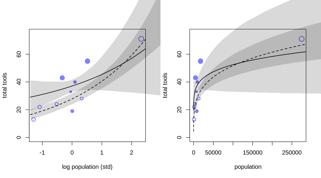
../_images/3012735790ffec4326f357e4c964e281c25fbd1ccca359e3cf3211da333c01b2.png

11M8. Revisit the data(Kline) islands example. This time drop Hawaii from the sample and refit the models. What changes do you observe?

Answer. The results of inference are significantly different, essentially changing the nature of the answer. The ‘outlier’ is relevant to what we conclude for both low and high contact cultures.

## R code 11.36
library(rethinking)
data(Kline)
d <- Kline

## R code 11.37
d$P <- scale(log(d$population))
d$contact_id <- ifelse(d$contact == "high", 2, 1)

## R code 11.45
dat <- list(
  T = d$total_tools,
  P = d$P,
  cid = d$contact_id
)

# interaction model
m11.10 <- ulam(
  alist(
    T ~ dpois(lambda),
    log(lambda) <- a[cid] + b[cid] * P,
    a[cid] ~ dnorm(3, 0.5),
    b[cid] ~ dnorm(0, 0.2)
  ),
  data = dat, chains = 4, log_lik = TRUE
)
flush.console()

k <- PSIS(m11.10, pointwise = TRUE)$k

iplot(function() {
  par(mfrow=c(1,2))
  ## R code 11.47
  plot(dat$P, dat$T,
    xlab = "log population (std)", ylab = "total tools",
    col = rangi2, pch = ifelse(dat$cid == 1, 1, 16), lwd = 2,
    ylim = c(0, 75), cex = 1 + normalize(k)
  )

  # set up the horizontal axis values to compute predictions at
  ns <- 100
  P_seq <- seq(from = -1.4, to = 3, length.out = ns)

  # predictions for cid=1 (low contact)
  lambda <- link(m11.10, data = data.frame(P = P_seq, cid = 1))
  lmu <- apply(lambda, 2, mean)
  lci <- apply(lambda, 2, PI)
  lines(P_seq, lmu, lty = 2, lwd = 1.5)
  shade(lci, P_seq, xpd = TRUE)

  # predictions for cid=2 (high contact)
  lambda <- link(m11.10, data = data.frame(P = P_seq, cid = 2))
  lmu <- apply(lambda, 2, mean)
  lci <- apply(lambda, 2, PI)
  lines(P_seq, lmu, lty = 1, lwd = 1.5)
  shade(lci, P_seq, xpd = TRUE)

  ## R code 11.48
  plot(d$population, d$total_tools,
    xlab = "population", ylab = "total tools",
    col = rangi2, pch = ifelse(dat$cid == 1, 1, 16), lwd = 2,
    ylim = c(0, 75), cex = 1 + normalize(k)
  )

  ns <- 100
  P_seq <- seq(from = -5, to = 3, length.out = ns)
  # 1.53 is sd of log(population)
  # 9 is mean of log(population)
  pop_seq <- exp(P_seq * 1.53 + 9)

  lambda <- link(m11.10, data = data.frame(P = P_seq, cid = 1))
  lmu <- apply(lambda, 2, mean)
  lci <- apply(lambda, 2, PI)
  lines(pop_seq, lmu, lty = 2, lwd = 1.5)
  shade(lci, pop_seq, xpd = TRUE)

  lambda <- link(m11.10, data = data.frame(P = P_seq, cid = 2))
  lmu <- apply(lambda, 2, mean)
  lci <- apply(lambda, 2, PI)
  lines(pop_seq, lmu, lty = 1, lwd = 1.5)
  shade(lci, pop_seq, xpd = TRUE)
}, ar=1.8)

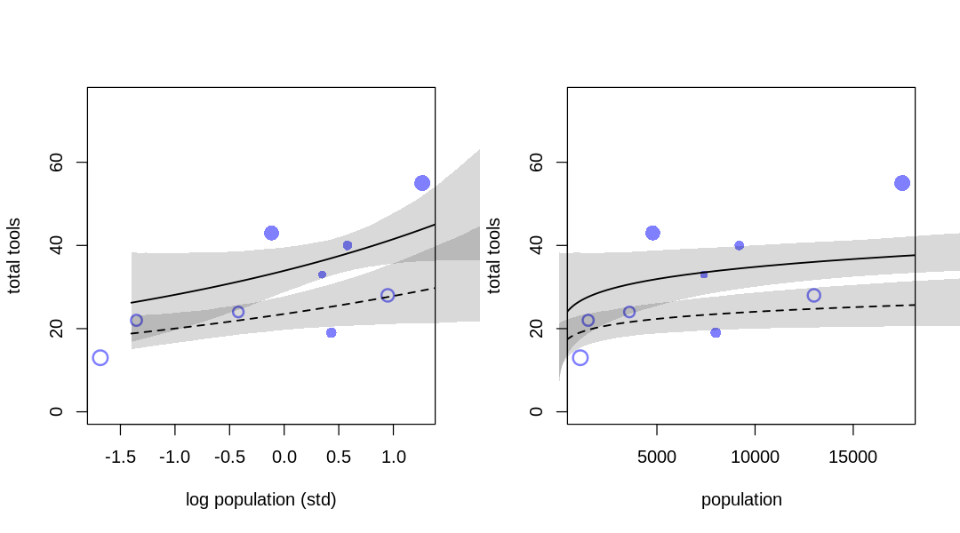
d_drop_hawaii <- subset(d, culture!='Hawaii')

# For some reason, we need to rescale and log to include the 'scale' attributes in the call to ulam.
d_drop_hawaii$P <- scale(log(d_drop_hawaii$population))
d_drop_hawaii$contact_id <- ifelse(d_drop_hawaii$contact == "high", 2, 1)

dat_drop_hawaii <- list(
  T = d_drop_hawaii$total_tools,
  P = d_drop_hawaii$P,
  cid = d_drop_hawaii$contact_id[1:9]
)

# interaction model
m_drop_hawaii <- ulam(
  alist(
    T ~ dpois(lambda),
    log(lambda) <- a[cid] + b[cid] * P,
    a[cid] ~ dnorm(3, 0.5),
    b[cid] ~ dnorm(0, 0.2)
  ),
  data = dat_drop_hawaii, chains = 4, log_lik = TRUE
)
flush.console()

k <- PSIS(m_drop_hawaii, pointwise = TRUE)$k

iplot(function() {
  par(mfrow=c(1,2))
  ## R code 11.47
  plot(dat_drop_hawaii$P, dat_drop_hawaii$T,
    xlab = "log population (std)", ylab = "total tools",
    col = rangi2, pch = ifelse(dat_drop_hawaii$cid == 1, 1, 16), lwd = 2,
    ylim = c(0, 75), cex = 1 + normalize(k)
  )

  # set up the horizontal axis values to compute predictions at
  ns <- 100
  P_seq <- seq(from = -1.4, to = 3, length.out = ns)

  # predictions for cid=1 (low contact)
  lambda <- link(m_drop_hawaii, data = data.frame(P = P_seq, cid = 1))
  lmu <- apply(lambda, 2, mean)
  lci <- apply(lambda, 2, PI)
  lines(P_seq, lmu, lty = 2, lwd = 1.5)
  shade(lci, P_seq, xpd = TRUE)

  # predictions for cid=2 (high contact)
  lambda <- link(m_drop_hawaii, data = data.frame(P = P_seq, cid = 2))
  lmu <- apply(lambda, 2, mean)
  lci <- apply(lambda, 2, PI)
  lines(P_seq, lmu, lty = 1, lwd = 1.5)
  shade(lci, P_seq, xpd = TRUE)

  ## R code 11.48
  plot(d_drop_hawaii$population, d_drop_hawaii$total_tools,
    xlab = "population", ylab = "total tools",
    col = rangi2, pch = ifelse(dat_drop_hawaii$cid == 1, 1, 16), lwd = 2,
    ylim = c(0, 75), cex = 1 + normalize(k)
  )

  ns <- 100
  P_seq <- seq(from = -5, to = 3, length.out = ns)
  # 1.53 is sd of log(population)
  # 9 is mean of log(population)
  pop_seq <- exp(P_seq * 1.53 + 9)

  lambda <- link(m_drop_hawaii, data = data.frame(P = P_seq, cid = 1))
  lmu <- apply(lambda, 2, mean)
  lci <- apply(lambda, 2, PI)
  lines(pop_seq, lmu, lty = 2, lwd = 1.5)
  shade(lci, pop_seq, xpd = TRUE)

  lambda <- link(m_drop_hawaii, data = data.frame(P = P_seq, cid = 2))
  lmu <- apply(lambda, 2, mean)
  lci <- apply(lambda, 2, PI)
  lines(pop_seq, lmu, lty = 1, lwd = 1.5)
  shade(lci, pop_seq, xpd = TRUE)
}, ar=1.8)

SAMPLING FOR MODEL '05013cdfcc1a8f52ceb5601ee475a98d' NOW (CHAIN 1).
Chain 1: 
Chain 1: Gradient evaluation took 1.4e-05 seconds
Chain 1: 1000 transitions using 10 leapfrog steps per transition would take 0.14 seconds.
Chain 1: Adjust your expectations accordingly!
Chain 1: 
Chain 1: 
Chain 1: Iteration:   1 / 1000 [  0%]  (Warmup)
Chain 1: Iteration: 100 / 1000 [ 10%]  (Warmup)
Chain 1: Iteration: 200 / 1000 [ 20%]  (Warmup)
Chain 1: Iteration: 300 / 1000 [ 30%]  (Warmup)
Chain 1: Iteration: 400 / 1000 [ 40%]  (Warmup)
Chain 1: Iteration: 500 / 1000 [ 50%]  (Warmup)
Chain 1: Iteration: 501 / 1000 [ 50%]  (Sampling)
Chain 1: Iteration: 600 / 1000 [ 60%]  (Sampling)
Chain 1: Iteration: 700 / 1000 [ 70%]  (Sampling)
Chain 1: Iteration: 800 / 1000 [ 80%]  (Sampling)
Chain 1: Iteration: 900 / 1000 [ 90%]  (Sampling)
Chain 1: Iteration: 1000 / 1000 [100%]  (Sampling)
Chain 1: 
Chain 1:  Elapsed Time: 0.015614 seconds (Warm-up)
Chain 1:                0.013301 seconds (Sampling)
Chain 1:                0.028915 seconds (Total)
Chain 1: 

SAMPLING FOR MODEL '05013cdfcc1a8f52ceb5601ee475a98d' NOW (CHAIN 2).
Chain 2: 
Chain 2: Gradient evaluation took 9e-06 seconds
Chain 2: 1000 transitions using 10 leapfrog steps per transition would take 0.09 seconds.
Chain 2: Adjust your expectations accordingly!
Chain 2: 
Chain 2: 
Chain 2: Iteration:   1 / 1000 [  0%]  (Warmup)
Chain 2: Iteration: 100 / 1000 [ 10%]  (Warmup)
Chain 2: Iteration: 200 / 1000 [ 20%]  (Warmup)
Chain 2: Iteration: 300 / 1000 [ 30%]  (Warmup)
Chain 2: Iteration: 400 / 1000 [ 40%]  (Warmup)
Chain 2: Iteration: 500 / 1000 [ 50%]  (Warmup)
Chain 2: Iteration: 501 / 1000 [ 50%]  (Sampling)
Chain 2: Iteration: 600 / 1000 [ 60%]  (Sampling)
Chain 2: Iteration: 700 / 1000 [ 70%]  (Sampling)
Chain 2: Iteration: 800 / 1000 [ 80%]  (Sampling)
Chain 2: Iteration: 900 / 1000 [ 90%]  (Sampling)
Chain 2: Iteration: 1000 / 1000 [100%]  (Sampling)
Chain 2: 
Chain 2:  Elapsed Time: 0.015469 seconds (Warm-up)
Chain 2:                0.013373 seconds (Sampling)
Chain 2:                0.028842 seconds (Total)
Chain 2: 

SAMPLING FOR MODEL '05013cdfcc1a8f52ceb5601ee475a98d' NOW (CHAIN 3).
Chain 3: 
Chain 3: Gradient evaluation took 9e-06 seconds
Chain 3: 1000 transitions using 10 leapfrog steps per transition would take 0.09 seconds.
Chain 3: Adjust your expectations accordingly!
Chain 3: 
Chain 3: 
Chain 3: Iteration:   1 / 1000 [  0%]  (Warmup)
Chain 3: Iteration: 100 / 1000 [ 10%]  (Warmup)
Chain 3: Iteration: 200 / 1000 [ 20%]  (Warmup)
Chain 3: Iteration: 300 / 1000 [ 30%]  (Warmup)
Chain 3: Iteration: 400 / 1000 [ 40%]  (Warmup)
Chain 3: Iteration: 500 / 1000 [ 50%]  (Warmup)
Chain 3: Iteration: 501 / 1000 [ 50%]  (Sampling)
Chain 3: Iteration: 600 / 1000 [ 60%]  (Sampling)
Chain 3: Iteration: 700 / 1000 [ 70%]  (Sampling)
Chain 3: Iteration: 800 / 1000 [ 80%]  (Sampling)
Chain 3: Iteration: 900 / 1000 [ 90%]  (Sampling)
Chain 3: Iteration: 1000 / 1000 [100%]  (Sampling)
Chain 3: 
Chain 3:  Elapsed Time: 0.015906 seconds (Warm-up)
Chain 3:                0.015114 seconds (Sampling)
Chain 3:                0.03102 seconds (Total)
Chain 3: 

SAMPLING FOR MODEL '05013cdfcc1a8f52ceb5601ee475a98d' NOW (CHAIN 4).
Chain 4: 
Chain 4: Gradient evaluation took 8e-06 seconds
Chain 4: 1000 transitions using 10 leapfrog steps per transition would take 0.08 seconds.
Chain 4: Adjust your expectations accordingly!
Chain 4: 
Chain 4: 
Chain 4: Iteration:   1 / 1000 [  0%]  (Warmup)
Chain 4: Iteration: 100 / 1000 [ 10%]  (Warmup)
Chain 4: Iteration: 200 / 1000 [ 20%]  (Warmup)
Chain 4: Iteration: 300 / 1000 [ 30%]  (Warmup)
Chain 4: Iteration: 400 / 1000 [ 40%]  (Warmup)
Chain 4: Iteration: 500 / 1000 [ 50%]  (Warmup)
Chain 4: Iteration: 501 / 1000 [ 50%]  (Sampling)
Chain 4: Iteration: 600 / 1000 [ 60%]  (Sampling)
Chain 4: Iteration: 700 / 1000 [ 70%]  (Sampling)
Chain 4: Iteration: 800 / 1000 [ 80%]  (Sampling)
Chain 4: Iteration: 900 / 1000 [ 90%]  (Sampling)
Chain 4: Iteration: 1000 / 1000 [100%]  (Sampling)
Chain 4: 
Chain 4:  Elapsed Time: 0.016163 seconds (Warm-up)
Chain 4:                0.012632 seconds (Sampling)
Chain 4:                0.028795 seconds (Total)
Chain 4: 

Some Pareto k values are very high (>1). Set pointwise=TRUE to inspect individual points.

../_images/5d63ad7caa2f849955f433cd24c8805c04c7612a72cc4043685fbf7b5b946705.png

SAMPLING FOR MODEL 'c5bf3fcd8c4a2bf16731479ec5cc9e70' NOW (CHAIN 1).
Chain 1: 
Chain 1: Gradient evaluation took 1.4e-05 seconds
Chain 1: 1000 transitions using 10 leapfrog steps per transition would take 0.14 seconds.
Chain 1: Adjust your expectations accordingly!
Chain 1: 
Chain 1: 
Chain 1: Iteration:   1 / 1000 [  0%]  (Warmup)
Chain 1: Iteration: 100 / 1000 [ 10%]  (Warmup)
Chain 1: Iteration: 200 / 1000 [ 20%]  (Warmup)
Chain 1: Iteration: 300 / 1000 [ 30%]  (Warmup)
Chain 1: Iteration: 400 / 1000 [ 40%]  (Warmup)
Chain 1: Iteration: 500 / 1000 [ 50%]  (Warmup)
Chain 1: Iteration: 501 / 1000 [ 50%]  (Sampling)
Chain 1: Iteration: 600 / 1000 [ 60%]  (Sampling)
Chain 1: Iteration: 700 / 1000 [ 70%]  (Sampling)
Chain 1: Iteration: 800 / 1000 [ 80%]  (Sampling)
Chain 1: Iteration: 900 / 1000 [ 90%]  (Sampling)
Chain 1: Iteration: 1000 / 1000 [100%]  (Sampling)
Chain 1: 
Chain 1:  Elapsed Time: 0.016739 seconds (Warm-up)
Chain 1:                0.014427 seconds (Sampling)
Chain 1:                0.031166 seconds (Total)
Chain 1: 

SAMPLING FOR MODEL 'c5bf3fcd8c4a2bf16731479ec5cc9e70' NOW (CHAIN 2).
Chain 2: 
Chain 2: Gradient evaluation took 9e-06 seconds
Chain 2: 1000 transitions using 10 leapfrog steps per transition would take 0.09 seconds.
Chain 2: Adjust your expectations accordingly!
Chain 2: 
Chain 2: 
Chain 2: Iteration:   1 / 1000 [  0%]  (Warmup)
Chain 2: Iteration: 100 / 1000 [ 10%]  (Warmup)
Chain 2: Iteration: 200 / 1000 [ 20%]  (Warmup)
Chain 2: Iteration: 300 / 1000 [ 30%]  (Warmup)
Chain 2: Iteration: 400 / 1000 [ 40%]  (Warmup)
Chain 2: Iteration: 500 / 1000 [ 50%]  (Warmup)
Chain 2: Iteration: 501 / 1000 [ 50%]  (Sampling)
Chain 2: Iteration: 600 / 1000 [ 60%]  (Sampling)
Chain 2: Iteration: 700 / 1000 [ 70%]  (Sampling)
Chain 2: Iteration: 800 / 1000 [ 80%]  (Sampling)
Chain 2: Iteration: 900 / 1000 [ 90%]  (Sampling)
Chain 2: Iteration: 1000 / 1000 [100%]  (Sampling)
Chain 2: 
Chain 2:  Elapsed Time: 0.015531 seconds (Warm-up)
Chain 2:                0.014058 seconds (Sampling)
Chain 2:                0.029589 seconds (Total)
Chain 2: 

SAMPLING FOR MODEL 'c5bf3fcd8c4a2bf16731479ec5cc9e70' NOW (CHAIN 3).
Chain 3: 
Chain 3: Gradient evaluation took 9e-06 seconds
Chain 3: 1000 transitions using 10 leapfrog steps per transition would take 0.09 seconds.
Chain 3: Adjust your expectations accordingly!
Chain 3: 
Chain 3: 
Chain 3: Iteration:   1 / 1000 [  0%]  (Warmup)
Chain 3: Iteration: 100 / 1000 [ 10%]  (Warmup)
Chain 3: Iteration: 200 / 1000 [ 20%]  (Warmup)
Chain 3: Iteration: 300 / 1000 [ 30%]  (Warmup)
Chain 3: Iteration: 400 / 1000 [ 40%]  (Warmup)
Chain 3: Iteration: 500 / 1000 [ 50%]  (Warmup)
Chain 3: Iteration: 501 / 1000 [ 50%]  (Sampling)
Chain 3: Iteration: 600 / 1000 [ 60%]  (Sampling)
Chain 3: Iteration: 700 / 1000 [ 70%]  (Sampling)
Chain 3: Iteration: 800 / 1000 [ 80%]  (Sampling)
Chain 3: Iteration: 900 / 1000 [ 90%]  (Sampling)
Chain 3: Iteration: 1000 / 1000 [100%]  (Sampling)
Chain 3: 
Chain 3:  Elapsed Time: 0.015582 seconds (Warm-up)
Chain 3:                0.014108 seconds (Sampling)
Chain 3:                0.02969 seconds (Total)
Chain 3: 

SAMPLING FOR MODEL 'c5bf3fcd8c4a2bf16731479ec5cc9e70' NOW (CHAIN 4).
Chain 4: 
Chain 4: Gradient evaluation took 8e-06 seconds
Chain 4: 1000 transitions using 10 leapfrog steps per transition would take 0.08 seconds.
Chain 4: Adjust your expectations accordingly!
Chain 4: 
Chain 4: 
Chain 4: Iteration:   1 / 1000 [  0%]  (Warmup)
Chain 4: Iteration: 100 / 1000 [ 10%]  (Warmup)
Chain 4: Iteration: 200 / 1000 [ 20%]  (Warmup)
Chain 4: Iteration: 300 / 1000 [ 30%]  (Warmup)
Chain 4: Iteration: 400 / 1000 [ 40%]  (Warmup)
Chain 4: Iteration: 500 / 1000 [ 50%]  (Warmup)
Chain 4: Iteration: 501 / 1000 [ 50%]  (Sampling)
Chain 4: Iteration: 600 / 1000 [ 60%]  (Sampling)
Chain 4: Iteration: 700 / 1000 [ 70%]  (Sampling)
Chain 4: Iteration: 800 / 1000 [ 80%]  (Sampling)
Chain 4: Iteration: 900 / 1000 [ 90%]  (Sampling)
Chain 4: Iteration: 1000 / 1000 [100%]  (Sampling)
Chain 4: 
Chain 4:  Elapsed Time: 0.018843 seconds (Warm-up)
Chain 4:                0.014995 seconds (Sampling)
Chain 4:                0.033838 seconds (Total)
Chain 4: 

Some Pareto k values are high (>0.5). Set pointwise=TRUE to inspect individual points.

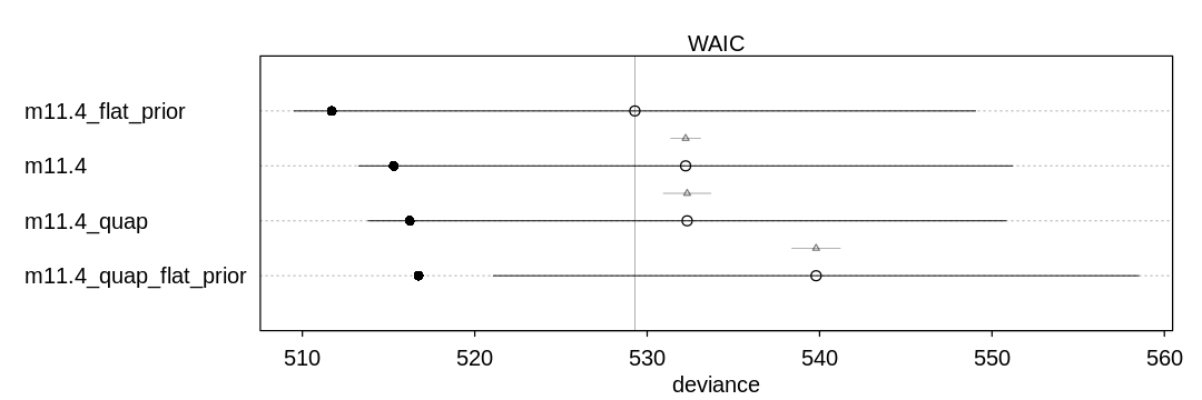
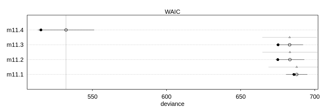
../_images/757ded2aed6a6ab2e0b5ce6cf74839d562a472dca1effe354eef784a1e6987cd.png

11H1. Use WAIC to compare the chimpanzee model that includes a unique intercept for each actor, m11.4 (page 330), to the simpler models fit in the same section. Interpret the results.

Answer. The last model (m11.4) does the best by far because it includes the actor predictor. The actor variable is highly predictive of the output; the big story of this experiment is handedness.

iplot(function() {
  plot(compare(m11.1, m11.2, m11.3, m11.4))
}, ar=3)

Warning message in compare(m11.1, m11.2, m11.3, m11.4):
“Not all model fits of same class.
This is usually a bad idea, because it implies they were fit by different algorithms.
Check yourself, before you wreck yourself.”

../_images/eb0d75c315d5510d5b18e9f10c3422e7a5fcc18e2d394ba5e1d3cbab6cd5ad43.png

11H2. The data contained in library(MASS);data(eagles) are records of salmon pirating attempts by Bald Eagles in Washington State. See ?eagles for details. While one eagle feeds, sometimes another will swoop in and try to steal the salmon from it. Call the feeding eagle the “victim” and the thief the “pirate.” Use the available data to build a binomial GLM of successful pirating attempts.

(a) Consider the following model: $$ \begin{align} \\ y_i & \sim Binomial(n_i, p_i) \\ logit(p_i) & = \alpha + \beta_P P_i + \beta_V V_i + \beta_A A_i \\ α & \sim Normal(0, 1.5) \\ \beta_P, \beta_V, \beta_A & \sim Normal(0, 0.5) \\ \end{align} $$

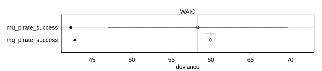
where $y$ is the number of successful attempts, $n$ is the total number of attempts, $P$ is a dummy variable indicating whether or not the pirate had large body size, $V$ is a dummy variable indicating whether or not the victim had large body size, and finally $A$ is a dummy variable indicating whether or not the pirate was an adult. Fit the model above to the eagles data, using both quap and ulam. Is the quadratic approximation okay?

Answer. The quadratic approximation is OK because this model includes pre-selected reasonable priors.

library(rethinking)
library(MASS)
data(eagles)
eag <- eagles
eag$Pi <- ifelse(eagles$P == "L", 1, 0)
eag$Vi <- ifelse(eagles$V == "L", 1, 0)
eag$Ai <- ifelse(eagles$A == "A", 1, 0)

mq_pirate_success <- quap(
  alist(
    y ~ dbinom(n, p),
    logit(p) <- a + b_P*Pi + b_V*Vi + b_A*Ai,
    a ~ dnorm(0, 1.5),
    b_P ~ dnorm(0, 0.5),
    b_V ~ dnorm(0, 0.5),
    b_A ~ dnorm(0, 0.5)
  ),
  data = eag
)

dat_eag <- list(
  n = eag$n,
  y = eag$y,
  Pi = eag$Pi,
  Vi = eag$Vi,
  Ai = eag$Ai
)

mu_pirate_success <- ulam(
  mq_pirate_success@formula,
  data = dat_eag, chains=4, cores=4, log_lik=TRUE
)

iplot(function() {
  plot(compare(mq_pirate_success, mu_pirate_success))
}, ar=4.5)

Warning message in compare(mq_pirate_success, mu_pirate_success):
“Not all model fits of same class.
This is usually a bad idea, because it implies they were fit by different algorithms.
Check yourself, before you wreck yourself.”

../_images/9265635a0b1c470d410ae341c0f67b91a3e8428042c81c54899d4e92d3e439fb.png

(b) Now interpret the estimates. If the quadratic approximation turned out okay, then it’s okay to use the quap estimates. Otherwise stick to ulam estimates. Then plot the posterior predictions. Compute and display both (1) the predicted probability of success and its 89% interval for each row (i) in the data, as well as (2) the predicted success count and its 89% interval. What different information does each type of posterior prediction provide?

Answer. The eagles data frame:

display(eagles)

A data.frame: 8 × 5
	y	n	P	A	V
	<int>	<int>	<fct>	<fct>	<fct>
1	17	24	L	A	L
2	29	29	L	A	S
3	17	27	L	I	L
4	20	20	L	I	S
5	1	12	S	A	L
6	15	16	S	A	S
7	0	28	S	I	L
8	1	4	S	I	S

This graph is from postcheck, as mentioned in the text. The documentation on this function isn’t too helpful; it’s easier to read the source code. In the following figure, the open circles ($mean in the raw data) represent the predicted probability of success and the vertical lines the 89% interval ($PI). The crosshairs represent the 89% interval of the predicted success count ($outPI). The purple dots are observed outcomes from the eagles data frame above. Notice outcomes are scaled to between zero and one; in case #1 the purple dot is at $17/24 \approx 0.7083$.

iplot(function() {
  result <- postcheck(mu_pirate_success)
  display_markdown("The raw data:")
  display(result)
})

The raw data:

$mean

0.710157399257729
0.927927363862875
0.562201465031564
0.86989774940961
0.328546090480074
0.716971297887675
0.203425159304023
0.571254516921082

$PI

A matrix: 2 × 8 of type dbl
5%	0.6109664	0.8873907	0.4534979	0.7992962	0.2183685	0.5978318	0.1289645	0.4277729
94%	0.8054732	0.9597742	0.6682283	0.9248639	0.4505562	0.8248680	0.2894805	0.7078469

$outPI

A matrix: 2 × 8 of type dbl
5%	0.5416667	0.8275862	0.3703704	0.7	0.08333333	0.5000	0.07142857	0.25
94%	0.8750000	1.0000000	0.7407407	1.0	0.58333333	0.9375	0.35714286	1.00

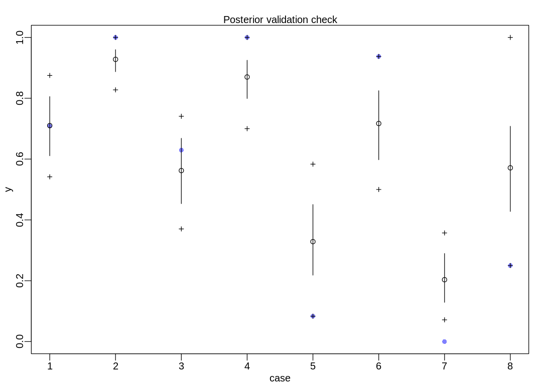
../_images/10982dfefee35db8563d00cf117f5d8c8f613efb05f04a2557953ef97ec4bed4.png

In part (1) we’re visualizing model parameters (including uncertainty). In part (2) we’re visualizing implied predictions on the outcome scale (including uncertainty) which indirectly includes the uncertainty in model parameters from the first part.

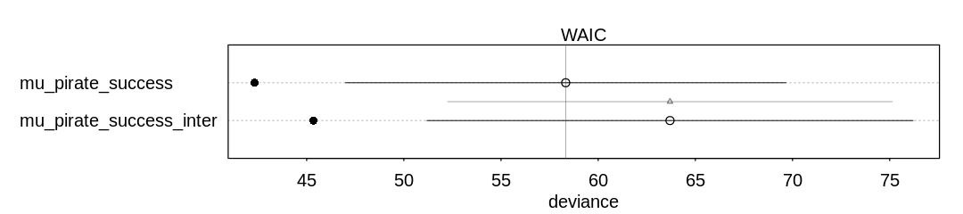
(c) Now try to improve the model. Consider an interaction between the pirate’s size and age (immature or adult). Compare this model to the previous one, using WAIC. Interpret.

Answer. The non-interaction model appears to do slightly better, but generally speaking the performance is almost the same. The interaction model is more complex (has more parameters) and that might slightly hurt its score.

eag$PirateTreatment <- 1 + eag$Pi + eag$Ai

dat_eag_inter <- list(
  n = eag$n,
  y = eag$y,
  PirateTreatment = eag$PirateTreatment,
  Vi = eag$Vi
)

mu_pirate_success_inter <- ulam(
  alist(
    y ~ dbinom(n, p),
    logit(p) <- a + b_t[PirateTreatment] + b_V*Vi,
    a ~ dnorm(0, 1.5),
    b_t[PirateTreatment] ~ dnorm(0, 0.5),
    b_V ~ dnorm(0, 0.5)
  ),
  data = dat_eag_inter, chains=4, cores=4, log_lik=TRUE
)

iplot(function() {
  plot(compare(mu_pirate_success_inter, mu_pirate_success))
}, ar=4.5)

../_images/edc96fcc3828238a64e8115a12378d91aa1c934c4bde405e8c4af1218f459255.png

11H4. The data contained in data(salamanders) are counts of salamanders (Plethodon elongatus) from 47 different 49-m² plots in northern California. The column SALAMAN is the count in each plot, and the columns PCTCOVER and FORESTAGE are percent of ground cover and age of trees in the plot, respectively. You will model SALAMAN as a Poisson variable.

(a) Model the relationship between density and percent cover, using a log-link (same as the example in the book and lecture). Use weakly informative priors of your choosing. Check the quadratic approximation again, by comparing quap to ulam. Then plot the expected counts and their 89% interval against percent cover. In which ways does the model do a good job? In which ways does it do a bad job?

Answer. The salamanders data frame:

data(salamanders)
display(salamanders)
sal <- salamanders
sal$StdPctCover <- scale(sal$PCTCOVER)

sal_dat <- list(
  S = sal$SALAMAN,
  StdPctCover = sal$StdPctCover
)

mq_sal <- quap(
  alist(
    S ~ dpois(lambda),
    log(lambda) <- a + b*StdPctCover,
    a ~ dnorm(3, 0.5),
    b ~ dnorm(0, 0.2)
  ), data = sal_dat
)

mu_sal <- ulam(
  mq_sal@formula,
  data = sal_dat, chains=4, cores=4, log_lik=TRUE
)

A data.frame: 47 × 4
SITE	SALAMAN	PCTCOVER	FORESTAGE
<int>	<int>	<int>	<int>
1	13	85	316
2	11	86	88
3	11	90	548
4	9	88	64
5	8	89	43
6	7	83	368
7	6	83	200
8	6	91	71
9	5	88	42
10	5	90	551
11	4	87	675
12	3	83	217
13	3	87	212
14	3	89	398
15	3	92	357
16	3	93	478
17	2	2	5
18	2	87	30
19	2	93	551
20	1	7	3
21	1	16	15
22	1	19	31
23	1	29	10
24	1	34	49
25	1	46	30
26	1	80	215
27	1	86	586
28	1	88	105
29	1	92	210
30	0	0	0
31	0	1	4
32	0	3	3
33	0	5	2
34	0	8	10
35	0	9	8
36	0	11	6
37	0	14	49
38	0	17	29
39	0	24	57
40	0	44	59
41	0	52	78
42	0	77	50
43	0	78	320
44	0	80	411
45	0	86	133
46	0	89	60
47	0	91	187

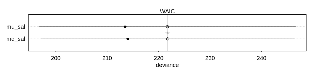
There doesn’t seem to be a difference between quap and ulam in inference:

iplot(function() {
  plot(compare(mu_sal, mq_sal))
}, ar=4.5)

pctc <- list(StdPctCover=scale(seq(0, 100)))
sims <- sim(mq_sal, data=pctc)

expectedSalCount.mu <- apply(sims, 2, mean)
expectedSalCount.PI <- apply(sims, 2, PI)
display_markdown("The raw data:")
display(expectedSalCount.mu)
display(expectedSalCount.PI)

iplot(function() {
  plot(pctc$StdPctCover, expectedSalCount.mu, ylim=c(0,12))
  shade(expectedSalCount.PI, pctc$StdPctCover)
  title("Expected salamander count")
})

Warning message in compare(mu_sal, mq_sal):
“Not all model fits of same class.
This is usually a bad idea, because it implies they were fit by different algorithms.
Check yourself, before you wreck yourself.”

../_images/42212c4534a88e62621786a4e41465f4114030ed7d5451af0aa0fadaaf1ac85a.png

The raw data:

0.763
0.753
0.74
0.881
0.865
0.848
0.834
0.899
0.888
0.945
0.938
0.95
1.037
0.988
0.994
0.99
1.053
1.066
1.131
1.119
1.113
1.191
1.204
1.225
1.28
1.309
1.34
1.377
1.39
1.373
1.508
1.504
1.466
1.531
1.632
1.584
1.629
1.669
1.731
1.711
1.868
1.808
1.957
1.996
1.971
2.12
2.013
2.1
2.135
2.136
2.289
2.319
2.32
2.506
2.589
2.509
2.484
2.597
2.626
2.771
2.826
2.927
2.981
2.961
3.045
3.14
3.182
3.286
3.401
3.54
3.537
3.544
3.638
3.782
3.878
3.901
4.059
3.94
4.287
4.172
4.333
4.57
4.576
4.755
4.802
4.895
5.061
5.234
5.22
5.388
5.399
5.629
5.759
5.975
6.124
6.161
6.275
6.458
6.461
6.739
7.016

A matrix: 2 × 101 of type dbl
5%	0	0	0	0	0	0	0	0	0	0	⋯	2	2	2	2	2	2	3	2.945	3	3
94%	2	2	2	3	3	3	3	3	3	3	⋯	10	10	10	11	11	11	11	11.000	12	12

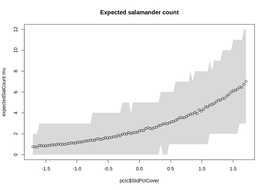
../_images/aa8bfcad55e4a7ff0c2b82519f9345da1f8d0348e19c87a0e94352336b2a1ca6.png

The model does well (is more certain) when it needs to guess lower numbers; when there are fewer salamanders when the ground cover is low. In general, though, it is uncertain about most of its predictions.

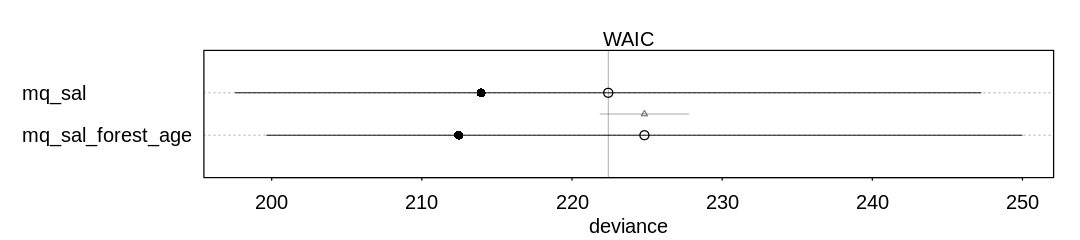
(b) Can you improve the model by using the other predictor, FORESTAGE? Try any models you think useful. Can you explain why FORESTAGE helps or does not help with prediction?

Answer. It doesn’t seem forest age helps much with prediction; it may be that forest age only predicts ground cover and so adds no extra information.

sal$StdForestAge <- scale(sal$FORESTAGE)
sal_dat <- list(
  S = sal$SALAMAN,
  StdPctCover = sal$StdPctCover,
  StdForestAge = sal$StdForestAge
)

mq_sal_forest_age <- quap(
  alist(
    S ~ dpois(lambda),
    log(lambda) <- a + b_c*StdPctCover + b_f*StdForestAge,
    a ~ dnorm(3, 0.5),
    b_c ~ dnorm(0, 0.2),
    b_f ~ dnorm(0, 0.2)
  ), data = sal_dat
)

iplot(function() {
  plot(compare(mq_sal, mq_sal_forest_age))
}, ar=4.5)

../_images/16c5f7f22805b4fb61907cd5334276ca30a431ad34cc8f520413a1ac062b2947.png

library(dagitty)

11H4. The data in data(NWOgrants) are outcomes for scientific funding applications for the Netherlands Organization for Scientific Research (NWO) from 2010-2012 (see van der Lee and Ellemers (2015) for data and context). These data have a very similar structure to the UCBAdmit data discussed in the chapter. I want you to consider a similar question: What are the total and indirect causal effects of gender on grant awards? Consider a mediation path (a pipe) through discipline. Draw the corresponding DAG and then use one or more binomial GLMs to answer the question. What is your causal interpretation? If NWO’s goal is to equalize rates of funding between men and women, what type of intervention would be most effective?

Answer. The NWOGrants data.frame:

data(NWOGrants)
display(NWOGrants)
nwo <- NWOGrants

A data.frame: 18 × 4
discipline	gender	applications	awards
<fct>	<fct>	<int>	<int>
Chemical sciences	m	83	22
Chemical sciences	f	39	10
Physical sciences	m	135	26
Physical sciences	f	39	9
Physics	m	67	18
Physics	f	9	2
Humanities	m	230	33
Humanities	f	166	32
Technical sciences	m	189	30
Technical sciences	f	62	13
Interdisciplinary	m	105	12
Interdisciplinary	f	78	17
Earth/life sciences	m	156	38
Earth/life sciences	f	126	18
Social sciences	m	425	65
Social sciences	f	409	47
Medical sciences	m	245	46
Medical sciences	f	260	29

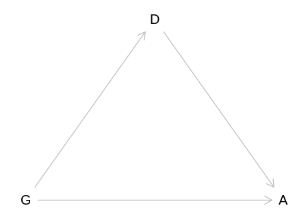
Reproduce the DAG from the text, where D now means discipline rather than department:

nwo_dag <- dagitty('
dag {
    bb="0,0,1,1"
    A [pos="0.500,0.400"]
    D [pos="0.300,0.300"]
    G [pos="0.100,0.400"]
    D -> A
    G -> A
    G -> D
}')
iplot(function() plot(nwo_dag), scale=10)

../_images/84a558c8bf920a0191915fd010d66f4ee2fec419cb14debb1ba77bb1f549f35c.png

For the total causal effect of gender on grant awards, do not condition on discipline:

nwo_dat <- list(
  awards = nwo$awards,
  applications = nwo$applications,
  gid = ifelse(as.character(nwo$gender) == "m", 1, 2)
)
m_nwo_tot <- quap(
  alist(
    awards ~ dbinom(applications, p),
    logit(p) <- a[gid],
    a[gid] ~ dnorm(0, 1.5)
  ),
  data = nwo_dat
)
iplot(function() {
  display_markdown("Raw data:")
  x <- precis(m_nwo_tot, depth = 2)
  display(x)
  plot(x, main="m_nwo_tot")
}, ar=4.5)

Raw data:

A precis: 2 × 4
	mean	sd	5.5%	94.5%
	<dbl>	<dbl>	<dbl>	<dbl>
a[1]	-1.531415	0.06462428	-1.634697	-1.428133
a[2]	-1.737434	0.08121384	-1.867230	-1.607639

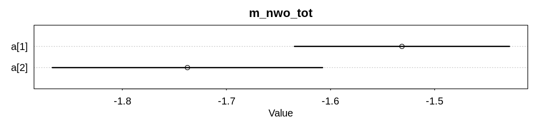
../_images/ad75ddc48badd5cb6cbf5d532a55ef3962d6fd749aae298ec91eb38268172bfb.png

These two coefficients are on the log-odds (parameter) scale, so the odds of a male getting an award from an application is about $exp(-1.53) = 0.217$ and the odds of a female about $exp(-1.74) = 0.176$. If it helps you can convert these absolute odds to probabilities with $p = o/(1+o)$.

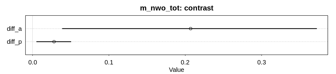
Lets also look at the relative performance of males to females (see Contrast (statistics)). As in the text we’ll do so on the logit and probability scale:

post <- extract.samples(m_nwo_tot)
diff_a <- post$a[,1] - post$a[,2]
diff_p <- inv_logit(post$a[,1]) - inv_logit(post$a[,2])
iplot(function() {
  display_markdown("Raw data:")
  x <- precis(list(diff_a=diff_a, diff_p=diff_p))
  display(x)
  plot(x, main="m_nwo_tot: contrast")
}, ar=4.5)

Raw data:

A precis: 2 × 5
	mean	sd	5.5%	94.5%	histogram
	<dbl>	<dbl>	<dbl>	<dbl>	<chr>
diff_a	0.20699102	0.1033998	0.039146118	0.37194581	▁▁▂▇▇▃▁▁
diff_p	0.02818477	0.0139731	0.005452507	0.05017562	▁▁▁▂▅▇▇▃▁▁▁

../_images/c7eaf7eca643ed5e4f4131fd16f6c450e91618c829aeeb2d997c24f32073928c.png

For the direct causal effect of gender on grant awards, condition on discipline:

nwo_dat$disc_id <- rep(1:9, each = 2)
m_nwo_dir <- quap(
  alist(
    awards ~ dbinom(applications, p),
    logit(p) <- a[gid] + delta[disc_id],
    a[gid] ~ dnorm(0, 1.5),
    delta[disc_id] ~ dnorm(0, 1.5)
  ),
  data = nwo_dat
)
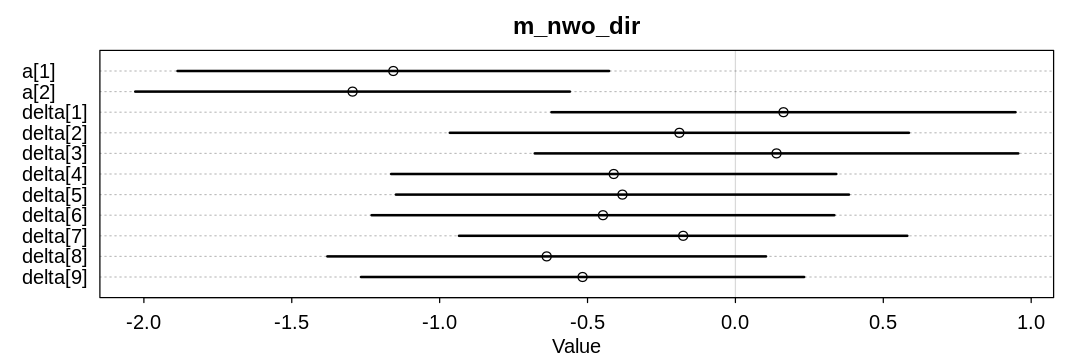
iplot(function() {
  display_markdown("Raw data:")
  x <- precis(m_nwo_dir, depth = 2)
  display(x)
  plot(x, main="m_nwo_dir")
}, ar=3)

post <- extract.samples(m_nwo_dir)
diff_a <- post$a[,1] - post$a[,2]
diff_p <- inv_logit(post$a[,1]) - inv_logit(post$a[,2])
iplot(function() {
  display_markdown("Raw data:")
  x <- precis(list(diff_a=diff_a, diff_p=diff_p))
  display(x)
  plot(x, main="m_nwo_dir: contrast")
}, ar=4.5)

Raw data:

A precis: 11 × 4
	mean	sd	5.5%	94.5%
	<dbl>	<dbl>	<dbl>	<dbl>
a[1]	-1.1567197	0.4565097	-1.8863105	-0.4271290
a[2]	-1.2944656	0.4597883	-2.0292961	-0.5596351
delta[1]	0.1624986	0.4908985	-0.6220521	0.9470492
delta[2]	-0.1894857	0.4856748	-0.9656879	0.5867165
delta[3]	0.1389274	0.5114875	-0.6785285	0.9563833
delta[4]	-0.4114458	0.4709091	-1.1640496	0.3411579
delta[5]	-0.3820280	0.4792310	-1.1479317	0.3838756
delta[6]	-0.4478024	0.4895143	-1.2301409	0.3345361
delta[7]	-0.1766539	0.4742538	-0.9346031	0.5812954
delta[8]	-0.6381023	0.4640408	-1.3797292	0.1035246
delta[9]	-0.5167944	0.4687254	-1.2659081	0.2323194

../_images/6ca0ad95403e1f88d04ef885d4a8c88c0caaed9d0cc4fba6ef93e05fd9987eea.png

Raw data:

A precis: 2 × 5
	mean	sd	5.5%	94.5%	histogram
	<dbl>	<dbl>	<dbl>	<dbl>	<chr>
diff_a	0.13732755	0.10669033	-0.033914612	0.30750179	▁▁▂▅▇▅▁▁▁
diff_p	0.02370068	0.01961388	-0.005735084	0.05587873	▁▁▂▇▇▃▁▁▁

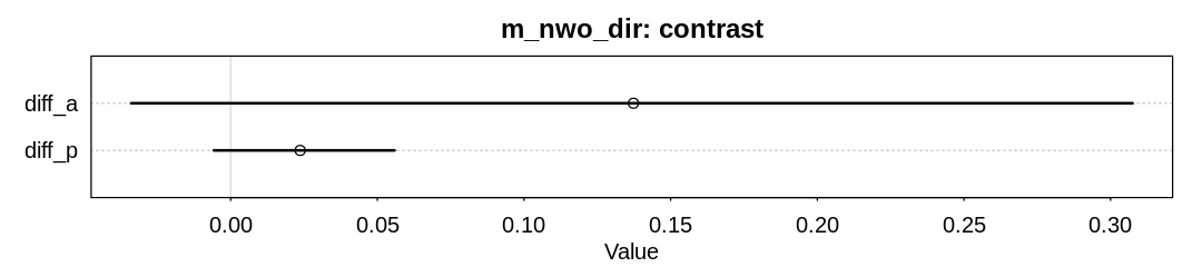
../_images/658f9d249e20b21b757cd587e2965062c7e0bdacfd5f1375adc06d4f66a916ec.png

Although the advantage for males has decreased, there is still some evidence for it.

One possible intervention is to increase funding to topics considered more valuable by females, assuming they prefer to do research in the areas they are applying. Another is to encourage females to get more involved (probably at a younger age) in the topics with more funding.

11H5. Suppose that the NWO Grants sample has an unobserved confound that influences both choice of discipline and the probability of an award. One example of such a confound could be the career stage of each applicant. Suppose that in some disciplines, junior scholars apply for most of the grants. In other disciplines, scholars from all career stages compete. As a result, career stage influences discipline as well as the probability of being awarded a grant. Add these influences to your DAG from the previous problem. What happens now when you condition on discipline? Does it provide an un-confounded estimate of the direct path from gender to an award? Why or why not? Justify your answer with the backdoor criterion. If you have trouble thinking this though, try simulating fake data, assuming your DAG is true. Then analyze it using the model from the previous problem. What do you conclude? Is it possible for gender to have a real direct causal influence but for a regression conditioning on both gender and discipline to suggest zero influence?

Answer. Reproducing the DAG from the text (where U is now career stage):

nwo_career_stage_dag <- dagitty('
dag {
    bb="0,0,1,1"
    A [pos="0.500,0.400"]
    D [pos="0.300,0.300"]
    G [pos="0.100,0.400"]
    U [latent,pos="0.500,0.300"]
    D -> A
    G -> A
    G -> D
    U -> D
    U -> A
}')
iplot(function() plot(nwo_career_stage_dag), scale=10)

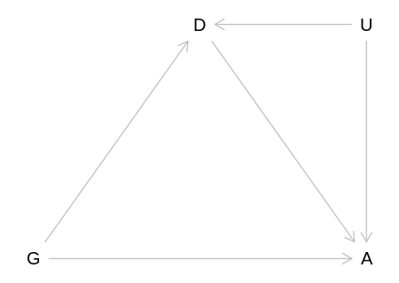
../_images/82610bb054231028fcd3b7419b7d00094626c8f73d8730cd00a335ded8ce719d.png

If we condition on D then we open the backdoor path ‘G -> D <- U -> A’, which could confound any causal inferences we make about the effect of gender on award. That is, we will induce a statistical association between G and A. This association could cancel out any direct causal influence of G on A.

# set.seed(145)
# n <- 100
# U <- rnorm(n)
# gid <- rbinom(n, 1, 0.5) + 1
# gender_to_disc_log_odds <- c(-0.2, 0.2)
# p_disc <- inv_logit(gender_to_disc_log_odds[gid] + U)
# disc_id <- rbinom(n, 1, p_disc) + 1
# gender_to_award_log_odds <- c(-1.5, -2)
# disc_to_award_log_odds <- c(0, 0)
# p_award <- inv_logit(gender_to_award_log_odds[gid] + U + disc_to_award_log_odds[disc_id])
# awards <- rbinom(n, 1, p_award)
#
# display_markdown("
# Imagine there are only two disciplines. Researchers with more scholarly experience tend to work in
# the second discipline, and females tend to work in the second discipline. If we know you're in the
# second discipline, and you got an award, then it's likely you got the award because you're
# experienced.
#
#
# We're assuming that discipline has no influence on award in this case; this assumption is not
# necessary for conditioning on discipline to connect (d-connect) gender and scholarly experience.
#
# G D U
# m 1 2
# f 1
# m 2 2
# f 2

11H6. The data in data(Primates301) are 301 primate species and associated measures. In this problem, you will consider how brain size is associated with social learning. There are three parts.

(a) Model the number of observations of social_learning for each species as a function of the log brain size. Use a Poisson distribution for the social_learning outcome variable. Interpret the resulting posterior.

Answer. The head of the Primates301 data.frame:

data(Primates301)
display(head(Primates301, n = 20L))
prim_inc <- Primates301
prim <- prim_inc[complete.cases(prim_inc$social_learning, prim_inc$brain, prim_inc$research_effort), ]

A data.frame: 20 × 16
	name	genus	species	subspecies	spp_id	genus_id	social_learning	research_effort	brain	body	group_size	gestation	weaning	longevity	sex_maturity	maternal_investment
	<fct>	<fct>	<fct>	<fct>	<int>	<int>	<int>	<int>	<dbl>	<dbl>	<dbl>	<dbl>	<dbl>	<dbl>	<dbl>	<dbl>
1	Allenopithecus_nigroviridis	Allenopithecus	nigroviridis	NA	1	1	0	6	58.02	4655.00	40.00	NA	106.15	276.0	NA	NA
2	Allocebus_trichotis	Allocebus	trichotis	NA	2	2	0	6	NA	78.09	1.00	NA	NA	NA	NA	NA
3	Alouatta_belzebul	Alouatta	belzebul	NA	3	3	0	15	52.84	6395.00	7.40	NA	NA	NA	NA	NA
4	Alouatta_caraya	Alouatta	caraya	NA	4	3	0	45	52.63	5383.00	8.90	185.92	323.16	243.6	1276.72	509.08
5	Alouatta_guariba	Alouatta	guariba	NA	5	3	0	37	51.70	5175.00	7.40	NA	NA	NA	NA	NA
6	Alouatta_palliata	Alouatta	palliata	NA	6	3	3	79	49.88	6250.00	13.10	185.42	495.60	300.0	1578.42	681.02
7	Alouatta_pigra	Alouatta	pigra	NA	7	3	0	25	51.13	8915.00	5.50	185.92	NA	240.0	NA	NA
8	Alouatta_sara	Alouatta	sara	NA	8	3	0	4	59.08	6611.04	NA	NA	NA	NA	NA	NA
9	Alouatta_seniculus	Alouatta	seniculus	NA	9	3	0	82	55.22	5950.00	7.90	189.90	370.04	300.0	1690.22	559.94
10	Aotus_azarai	Aotus	azarai	NA	10	4	0	22	20.67	1205.00	4.10	NA	229.69	NA	NA	NA
11	Aotus_azarai_boliviensis	Aotus	azarai	boliviensis	11	4	NA	NA	NA	NA	NA	NA	NA	NA	NA	NA
12	Aotus_brumbacki	Aotus	brumbacki	NA	12	4	0	NA	NA	NA	NA	NA	NA	NA	NA	NA
13	Aotus_infulatus	Aotus	infulatus	NA	13	4	0	6	NA	NA	NA	NA	NA	NA	NA	NA
14	Aotus_lemurinus	Aotus	lemurinus	NA	14	4	0	16	16.30	734.00	NA	132.23	74.57	216.0	755.15	206.80
15	Aotus_lemurinus_griseimembra	Aotus	lemurinus	griseimembra	15	4	NA	NA	NA	NA	NA	NA	NA	NA	NA	NA
16	Aotus_nancymaae	Aotus	nancymaae	NA	16	4	0	5	NA	791.03	4.00	NA	NA	NA	NA	NA
17	Aotus_nigriceps	Aotus	nigriceps	NA	17	4	0	1	NA	958.00	3.30	NA	NA	NA	NA	NA
18	Aotus_trivirgatus	Aotus	trivirgatus	NA	18	4	0	58	16.85	989.00	3.15	133.47	76.21	303.6	736.60	209.68
19	Aotus_vociferans	Aotus	vociferans	NA	19	4	0	12	NA	703.00	3.30	NA	NA	NA	NA	NA
20	Archaeolemur_majori	Archaeolemur	majori	NA	20	5	NA	NA	NA	NA	NA	NA	NA	NA	NA	NA

After filtering for complete cases:

display(head(prim, n = 20L))

brain_dat <- list(
  SocialLearning = prim$social_learning,
  LogBrain = log(prim$brain)
)

mq_brain_size <- quap(
  alist(
    SocialLearning ~ dpois(lambda),
    log(lambda) <- a + b * LogBrain,
    a ~ dnorm(3, 0.5),
    b ~ dnorm(0, 0.2)
  ),
  data = brain_dat
)

mu_brain_size <- ulam(
  mq_brain_size@formula,
  data = brain_dat, chains = 4, cores = 4, log_lik = TRUE
)

A data.frame: 20 × 16
	name	genus	species	subspecies	spp_id	genus_id	social_learning	research_effort	brain	body	group_size	gestation	weaning	longevity	sex_maturity	maternal_investment
	<fct>	<fct>	<fct>	<fct>	<int>	<int>	<int>	<int>	<dbl>	<dbl>	<dbl>	<dbl>	<dbl>	<dbl>	<dbl>	<dbl>
1	Allenopithecus_nigroviridis	Allenopithecus	nigroviridis	NA	1	1	0	6	58.02	4655.00	40.00	NA	106.15	276.0	NA	NA
3	Alouatta_belzebul	Alouatta	belzebul	NA	3	3	0	15	52.84	6395.00	7.40	NA	NA	NA	NA	NA
4	Alouatta_caraya	Alouatta	caraya	NA	4	3	0	45	52.63	5383.00	8.90	185.92	323.16	243.6	1276.72	509.08
5	Alouatta_guariba	Alouatta	guariba	NA	5	3	0	37	51.70	5175.00	7.40	NA	NA	NA	NA	NA
6	Alouatta_palliata	Alouatta	palliata	NA	6	3	3	79	49.88	6250.00	13.10	185.42	495.60	300.0	1578.42	681.02
7	Alouatta_pigra	Alouatta	pigra	NA	7	3	0	25	51.13	8915.00	5.50	185.92	NA	240.0	NA	NA
8	Alouatta_sara	Alouatta	sara	NA	8	3	0	4	59.08	6611.04	NA	NA	NA	NA	NA	NA
9	Alouatta_seniculus	Alouatta	seniculus	NA	9	3	0	82	55.22	5950.00	7.90	189.90	370.04	300.0	1690.22	559.94
10	Aotus_azarai	Aotus	azarai	NA	10	4	0	22	20.67	1205.00	4.10	NA	229.69	NA	NA	NA
14	Aotus_lemurinus	Aotus	lemurinus	NA	14	4	0	16	16.30	734.00	NA	132.23	74.57	216.0	755.15	206.80
18	Aotus_trivirgatus	Aotus	trivirgatus	NA	18	4	0	58	16.85	989.00	3.15	133.47	76.21	303.6	736.60	209.68
22	Arctocebus_calabarensis	Arctocebus	calabarensis	NA	22	6	0	1	6.92	309.00	1.00	133.74	109.26	156.0	298.91	243.00
23	Ateles_belzebuth	Ateles	belzebuth	NA	23	7	0	12	117.02	8167.00	14.50	138.20	NA	336.0	NA	NA
24	Ateles_fusciceps	Ateles	fusciceps	NA	24	7	0	4	114.24	9025.00	NA	224.70	482.70	288.0	1799.68	707.40
25	Ateles_geoffroyi	Ateles	geoffroyi	NA	25	7	2	58	105.09	7535.00	42.00	226.37	816.35	327.6	2104.57	1042.72
26	Ateles_paniscus	Ateles	paniscus	NA	26	7	0	30	103.85	8280.00	20.00	228.18	805.41	453.6	2104.57	1033.59
28	Avahi_laniger	Avahi	laniger	NA	28	8	0	10	9.86	1207.00	2.00	136.15	149.15	NA	NA	285.30
29	Avahi_occidentalis	Avahi	occidentalis	NA	29	8	0	6	7.95	801.00	3.00	NA	NA	NA	NA	NA
32	Bunopithecus_hoolock	Bunopithecus	hoolock	NA	32	10	0	24	110.68	6728.00	3.20	232.50	635.13	NA	2689.08	867.63
33	Cacajao_calvus	Cacajao	calvus	NA	33	11	0	11	76.00	3165.00	23.70	180.00	339.29	324.0	1262.74	519.29

Warning message:
“Bulk Effective Samples Size (ESS) is too low, indicating posterior means and medians may be unreliable.
Running the chains for more iterations may help. See
https://mc-stan.org/misc/warnings.html#bulk-ess”

Warning message:
“Tail Effective Samples Size (ESS) is too low, indicating posterior variances and tail quantiles may be unreliable.
Running the chains for more iterations may help. See
https://mc-stan.org/misc/warnings.html#tail-ess”

Use func=PSIS to generate warnings for high Pareto k values.

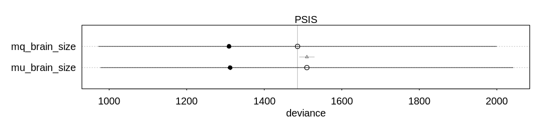
If you look at the data, you’ll see some classes (e.g. Gorillas and Chimpanzees) have orders of magnitude more study and more social learning examples than other species.

iplot(function()
  plot(compare(mq_brain_size, mu_brain_size, func=PSIS))
, ar=4.5)

iplot(function() {
  display_markdown("<br/>Raw data:")
  x <- precis(mq_brain_size)
  display(x)
  plot(x, main="mq_brain_size")
}, ar=4.5)

Warning message in compare(mq_brain_size, mu_brain_size, func = PSIS):
“Not all model fits of same class.
This is usually a bad idea, because it implies they were fit by different algorithms.
Check yourself, before you wreck yourself.”

Some Pareto k values are very high (>1). Set pointwise=TRUE to inspect individual points.

Some Pareto k values are very high (>1). Set pointwise=TRUE to inspect individual points.

../_images/248e93f5e67c2e3675c42d346a3fbaf153d60db31271124471a500bd8237dbf6.png

Raw data:

A precis: 2 × 4
	mean	sd	5.5%	94.5%
	<dbl>	<dbl>	<dbl>	<dbl>
a	-5.687636	0.24026506	-6.071626	-5.303646
b	1.563520	0.04787613	1.487005	1.640035

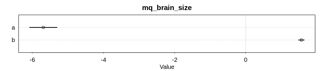
../_images/506f3f3cb3b744b82e712e1517a7010081e3053d512818a1e0e35024f4be6c1e.png

Although the model is confident in the b coefficient, the wide error bars on the WAIC scores indicate the out-of-sample performance may be much worse.

Still, in the context of this model it appears there is an association between brain size and social learning. For every unit increase in LogBrain i.e. for every order of magnitude increase in brain size we should see an exponential increase in examples of social learning. If we let $b = 1.5$ then for every order of magnitude we’ll see about $exp(1.5) \approx 4.5$ more examples of social learning.

(b) Some species are studied much more than others. So the number of reported instances of social_learning could be a product of research effort. Use the research_effort variable, specifically its logarithm, as an additional predictor variable. Interpret the coefficient for log research_effort. How does this model differ from the previous one?

brain_dat$LogResearchEffort <- log(prim$research_effort)

mq_brain_research <- quap(
  alist(
    SocialLearning ~ dpois(lambda),
    log(lambda) <- a + b * LogBrain + d * LogResearchEffort,
    a ~ dnorm(3, 0.5),
    b ~ dnorm(0, 0.2),
    d ~ dnorm(0, 0.2)
  ),
  data = brain_dat
)

mu_brain_research <- ulam(
  mq_brain_research@formula,
  data = brain_dat, chains = 4, cores = 4, log_lik = TRUE
)

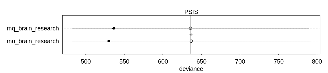
Again, use func=PSIS to generate warnings for high Pareto k values:

iplot(function()
  plot(compare(mq_brain_research, mu_brain_research, func=PSIS))
, ar=4.5)

iplot(function() {
  display_markdown("<br/>Raw data:")
  x <- precis(mq_brain_research)
  display(x)
  plot(x, main="mq_brain_research")
}, ar=4.5)

Warning message in compare(mq_brain_research, mu_brain_research, func = PSIS):
“Not all model fits of same class.
This is usually a bad idea, because it implies they were fit by different algorithms.
Check yourself, before you wreck yourself.”

Some Pareto k values are very high (>1). Set pointwise=TRUE to inspect individual points.

Some Pareto k values are very high (>1). Set pointwise=TRUE to inspect individual points.

../_images/7a9874d2f0ad9d61526408e1a7eb1b256c594f958e90b474cec88a972af19cb2.png

Raw data:

A precis: 3 × 4
	mean	sd	5.5%	94.5%
	<dbl>	<dbl>	<dbl>	<dbl>
a	-5.2692633	0.20355690	-5.5945865	-4.9439400
b	0.2326161	0.05079163	0.1514412	0.3137909
d	1.3094503	0.05033045	1.2290125	1.3898881

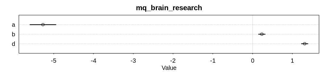
../_images/a0719fae03f30b84757d8dda25f8913d1874fa5d817e614e0fa98104d68a71d8.png

Answer. When we start to condition on research effort, the influence of brain size drops dramatically (to about 0.2 from 1.5).

(c) Draw a DAG to represent how you think the variables social_learning, brain, and research_effort interact. Justify the DAG with the measured associations in the two models above (and any other models you used).

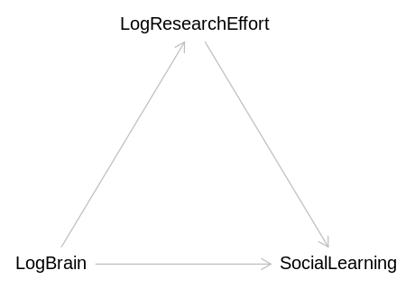
Answer. It seems likely we were looking at the total causal effect of LogBrain in the first model, and the direct causal effect in the second.

brain_social_learning_dag <- dagitty('
dag {
    bb="0,0,1,1"
    LogBrain [pos="0.100,0.400"]
    LogResearchEffort [pos="0.300,0.300"]
    SocialLearning [pos="0.500,0.400"]
    LogBrain -> SocialLearning
    LogBrain -> LogResearchEffort
    LogResearchEffort -> SocialLearning
}')
iplot(function() plot(brain_social_learning_dag), scale=10)

../_images/fcc113feca431ec963350aac85682c2b60802fd4f1b6ebb219867a1bbe39d22b.png