Practice: Chp. 16

source("iplot.R")
suppressPackageStartupMessages(library(rethinking))

16E1. What are some disadvantages of generalized linear models (GLMs)?

Answer. Parameters are often not interpretable, and therefore it is difficult to set priors on them.

When predictions disagree with observations, an understanding of the model provides a path to improving it rather than simply tuning epicycles. That is, we have a path to do something about errors.

16E2. Can you think of one or more famous scientific models which do not have the additive structure of a GLM?

Answer. All of Maxwell’s equations, which are based on differential equations.

16E3. Some models do not look like GLMs at first, but can be transformed through a logarithm into an additive combination of terms. Do you know any scientific models like this?

Answer. Theories that are based on addition can be modeled directly in a GLM. Theories that are based on multiplication would require a logarithm. Newton’s law of universal gravitation is based on the multiplication of two masses.

16M1. Modify the cylinder height model, m16.1, so that the exponent 3 on height is instead a free parameter. Do you recover the value of 3 or not? Plot the posterior predictions for the new model. How do they differ from those of m16.1?

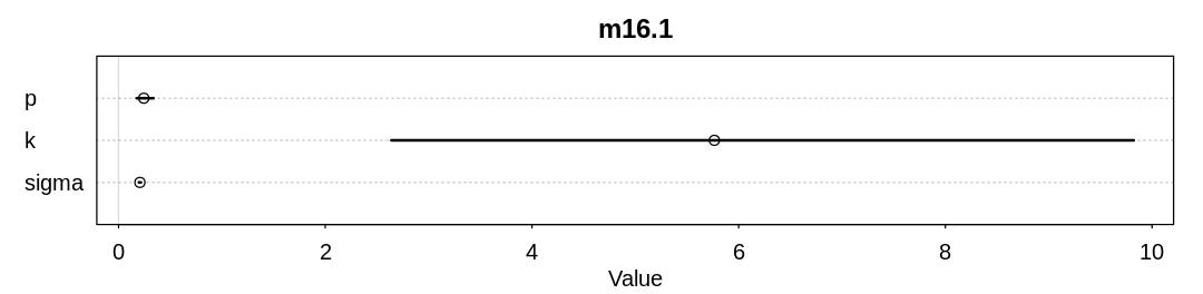
Answer. First, let’s reproduce results for m16.1:

load.d16m1 <- function() {
  data(Howell1)
  d <- Howell1
  
  # scale observed variables
  d$w <- d$weight / mean(d$weight)
  d$h <- d$height / mean(d$height)
  return(d)
}
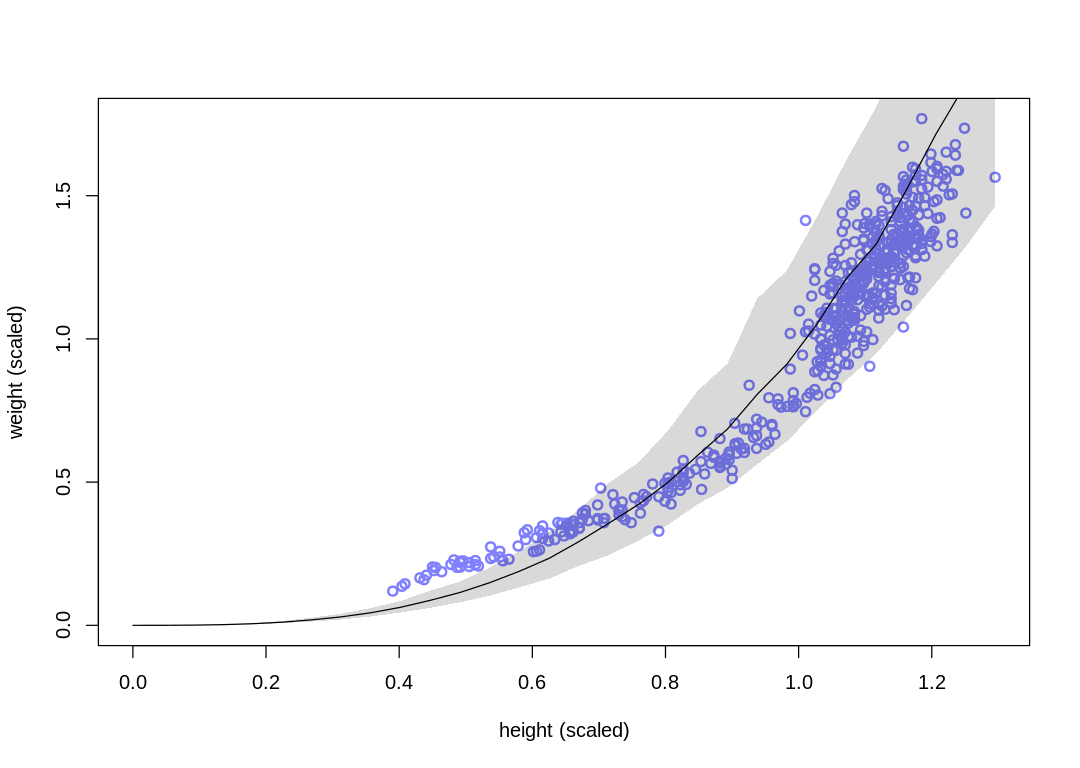
vcpp <- function(mc, d) {
  h_seq <- seq(from = 0, to = max(d$h), length.out = 30)
  w_sim <- sim(mc, data = list(h = h_seq))
  mu_mean <- apply(w_sim, 2, mean)
  w_CI <- apply(w_sim, 2, PI)
  iplot(function() {
    plot(d$h, d$w,
      xlim = c(0, max(d$h)), ylim = c(0, max(d$w)), col = rangi2,
      lwd = 2, xlab = "height (scaled)", ylab = "weight (scaled)"
    )
    lines(h_seq, mu_mean)
    shade(w_CI, h_seq)
  })
}
fm16m1 <- function(d) {
  m16.1 <- ulam(
    alist(
      w ~ dlnorm(mu, sigma),
      exp(mu) <- 3.141593 * k * p^2 * h^3,
      p ~ beta(2, 18),
      k ~ exponential(0.5),
      sigma ~ exponential(1)
    ),
    data = d, chains = 4, cores = 4
  )
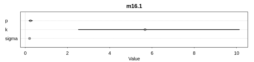
  display_precis(m16.1, "m16.1", ar=4.0)
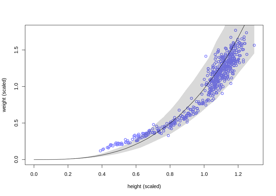
  vcpp(m16.1, d)
  return(m16.1)
}
d <- load.d16m1()
m16.1 <- fm16m1(d)

Raw data (following plot):

      mean      sd          5.5%      94.5%      n_eff    Rhat4   
p     0.2486417 0.057684255 0.1725625  0.3457837 431.6007 1.003236
k     5.6724141 2.614608076 2.5200429 10.1366305 422.3876 1.005251
sigma 0.2067652 0.006353465 0.1965858  0.2173697 743.4132 1.005612

Fitting the new model with a parameterized exponent:

fm3exp <- function(d) {
  m3exp <- ulam(
    alist(
      w ~ dlnorm(mu, sigma),
      exp(mu) <- 3.141593 * k * p^2 * h^he,
      p ~ beta(2, 18),
      k ~ exponential(0.5),
      he ~ dexp(0.5),
      sigma ~ exponential(1)
    ),
    data = d, chains = 4, cores = 4
  )
  display_precis(m3exp, "m3exp", ar=4.0)
  vcpp(m3exp, d)
  return(m3exp)
}
m3exp <- fm3exp(d)

Warning message:
“There were 21 transitions after warmup that exceeded the maximum treedepth. Increase max_treedepth above 10. See
https://mc-stan.org/misc/warnings.html#maximum-treedepth-exceeded”

Warning message:
“Examine the pairs() plot to diagnose sampling problems
”

Raw data (following plot):

      mean      sd          5.5%      94.5%      n_eff     Rhat4   
p     0.2495159 0.059390867 0.1675188  0.3492179  527.1705 1.000874
k     5.6170355 2.765135251 2.4263448 10.5751250  576.4607 1.000557
he    2.3241583 0.023079839 2.2882454  2.3609120 1112.5001 1.003386
sigma 0.1264380 0.003843978 0.1203479  0.1329253 1131.9201 1.003434

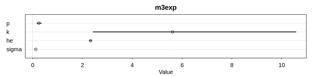
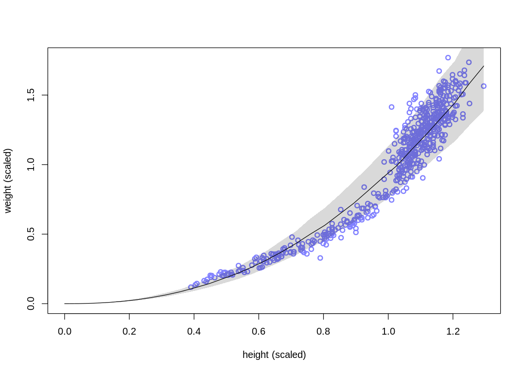
The new model fits the data better in the range of children, at some cost to the fit in the range of adults. In general it fits more closely; notice the change in the sigma estimate.

16M2. Conduct a prior predictive simulation for the cylinder height model. Begin with the priors in the chapter. Do these produce reasonable prior height distributions? If not, which modifications do you suggest?

ERROR:

Do these produce reasonable prior height distributions?

We’re predicting weight, so the author likely meant reasonable weight distributions.

pp16m2 <- function(p_sim, k_sim) {
  h_seq <- seq(from=0, to=1.0, length.out=30)
  iplot(function() {
    plot(NULL, NULL,
      xlim = c(0, max(h_seq)), ylim = c(0, 1.0), col = rangi2,
      lwd = 2, xlab = "height (scaled)", ylab = "weight (scaled)", main="Cylinder Prior Predictive"
    )
    for (i in 1:length(p_sim)) {
      mu_median <- pi * k_sim[i] * p_sim[i]^2 * h_seq ^ 3
      d <- data.frame(h=h_seq, w=mu_median)
      lines(h_seq, mu_median)
    }
  })
}
s16m2 <- function() {
  set.seed(7)
  N <- 20
  p_sim <- rbeta(N, shape1=2, shape2=18)
  k_sim <- rexp(N, rate=0.5)
  pp16m2(p_sim, k_sim)
}
s16m2()

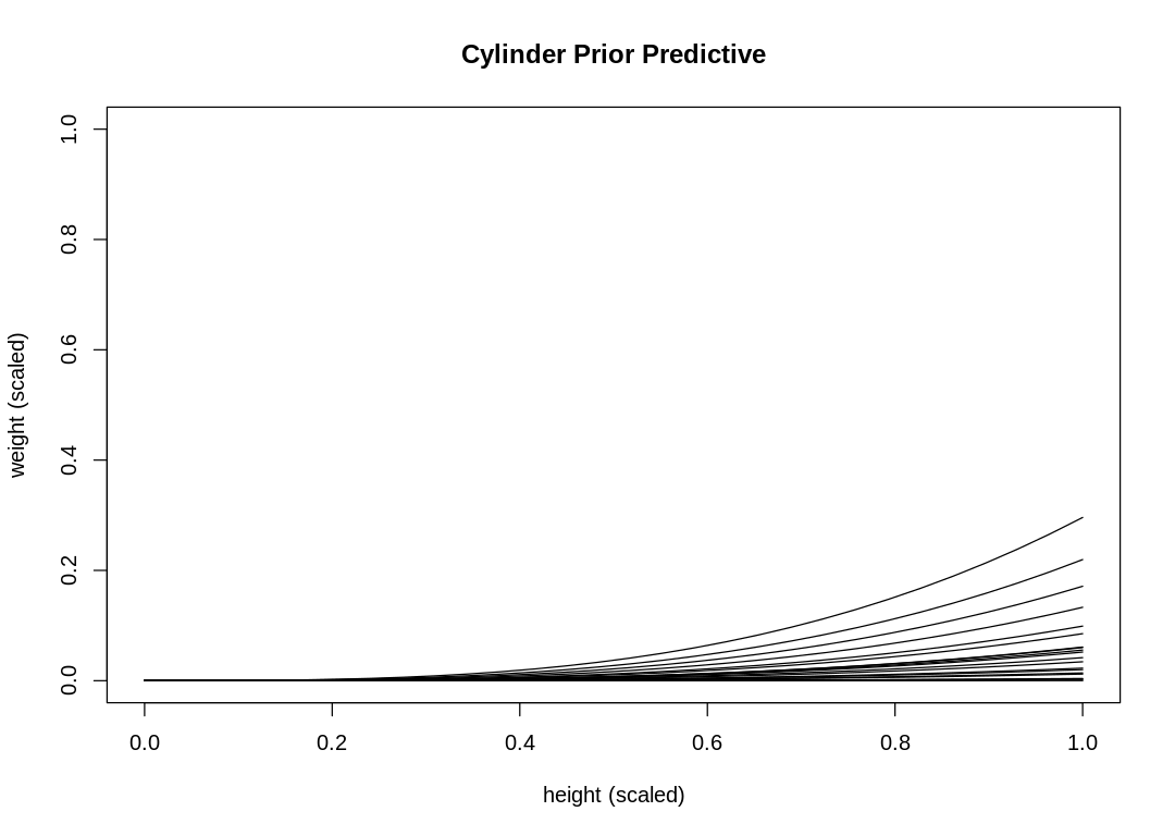
These priors do not produce a reasonable weight distribution; we rarely produce a sample that touches the maximum weight.

Part of the reason for this is that the exponential distribution puts a lot of probability near zero. This leads to many more curves on the lower end of the distribution than the upper end. To fix this, use a LogNormal distribution instead.

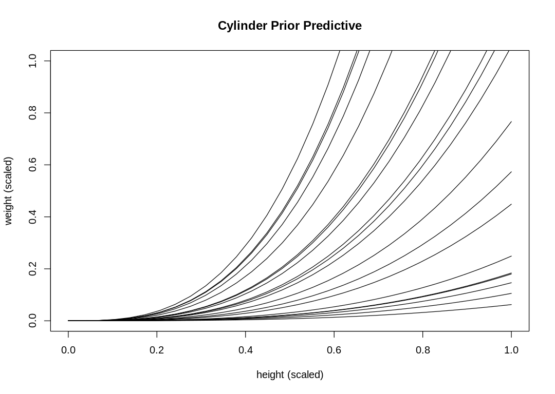
Another part of the reason is that we were not careful selecting the k prior. Returning to the equation we used to pick k in the text:

\[ 1 = k \pi p^2 1^3 \]

Solving for k and assuming we set p to 0.1:

\[ k = \frac{1}{\pi p^2} = \frac{1}{\pi \cdot 0.1^2} \approx 31.8 \]

Set k to 32 and use a LogNormal prior to produce a better simulation:

s16m2a <- function() {
  set.seed(7)
  N <- 20
  p_sim <- rbeta(N, shape1=2, shape2=18)
  k_sim <- rlnorm(N, meanlog=log(30), sdlog=0.1)
  pp16m2(p_sim, k_sim)
}
s16m2a()

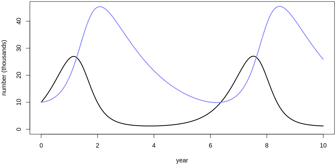
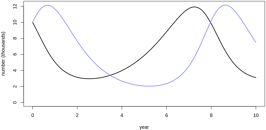
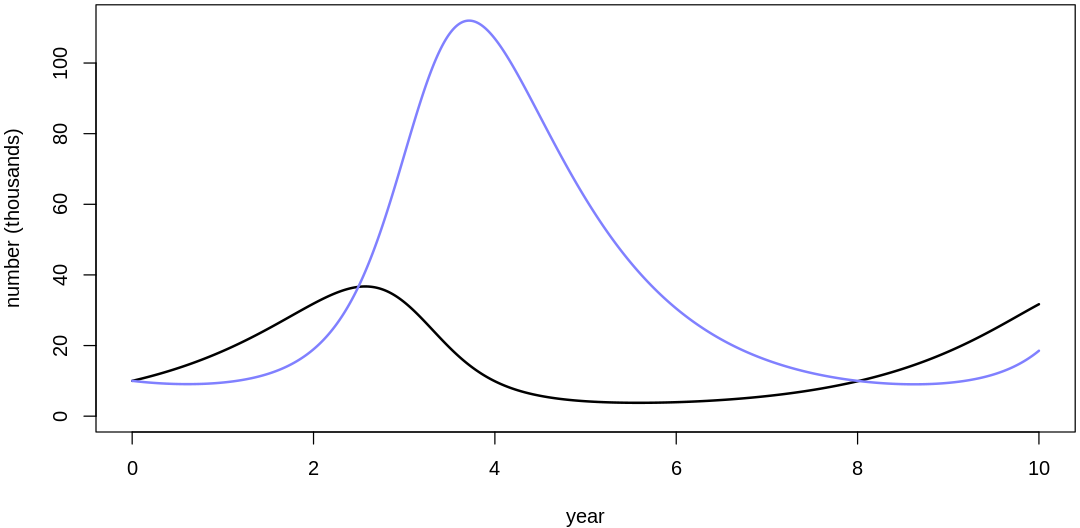
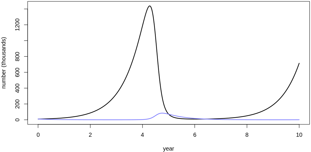
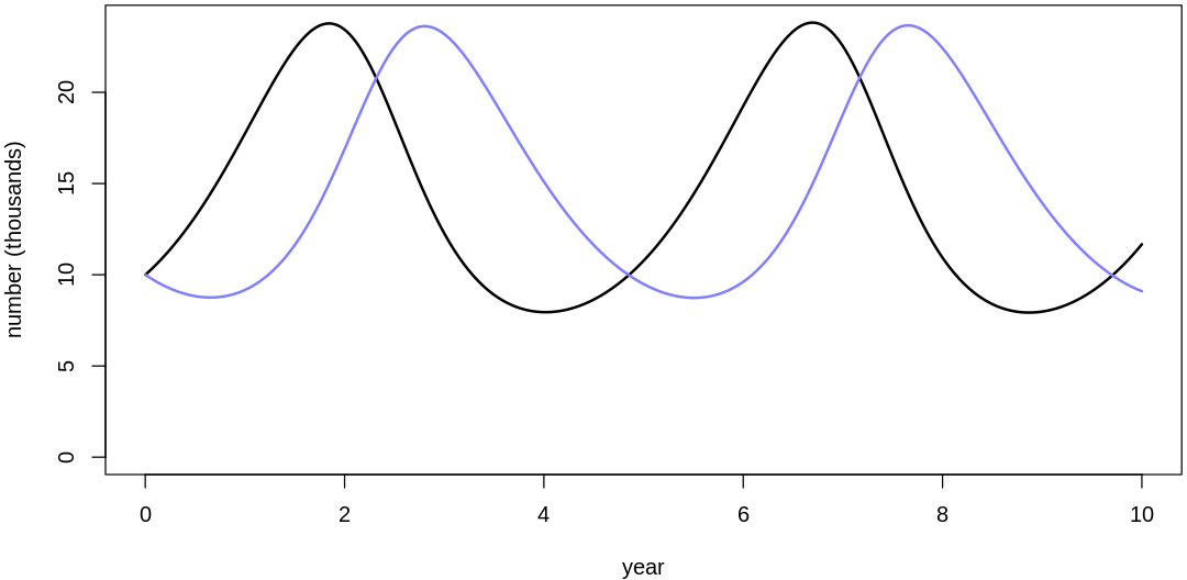
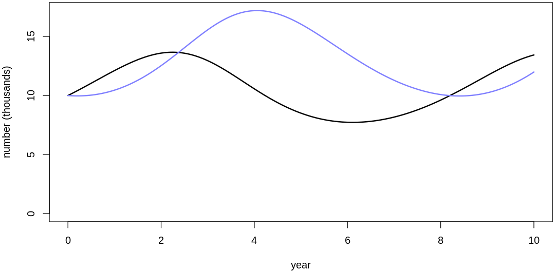
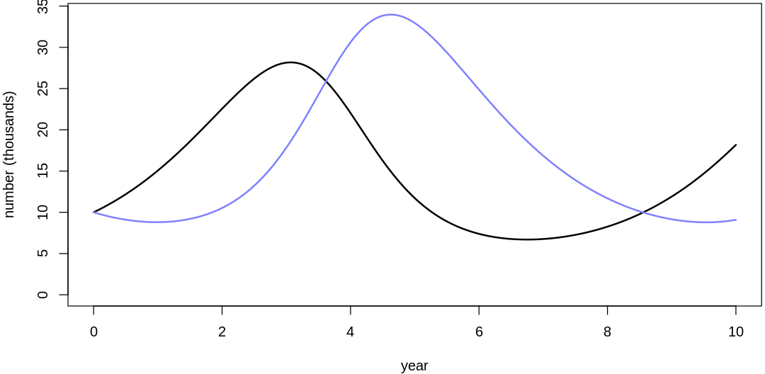
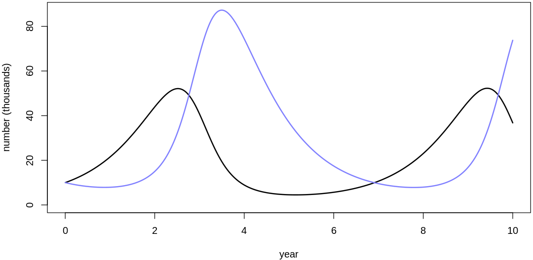
16M3. Use prior predictive simulations to investigate the lynx-hare model. Begin with the priors in the chapter. Which population dynamics do these produce? Can you suggest any improvements to the priors, on the basis of your simulations?

Answer. Sampling only ten simulations from the priors:

sim.pred.prey <- function(n_steps, init, theta, dt = 0.002) {
  # Euler method; exactly the same as `sim_lynx_hare` in the text.
  Pred <- rep(NA, n_steps)
  Prey <- rep(NA, n_steps)
  Pred[1] <- init[1]
  Prey[1] <- init[2]
  for (i in 2:n_steps) {
    Prey[i] <- Prey[i - 1] + dt * Prey[i - 1] * (theta[1] - theta[2] * Pred[i - 1])
    Pred[i] <- Pred[i - 1] + dt * Pred[i - 1] * (theta[3] * Prey[i - 1] - theta[4])
  }
  return(cbind(Pred, Prey))
}
pp16m3 <- function(theta) {
  iplot(function() {
    par(mar = c(4.0, 4.0, 0.2, 0.2))
    n_sim <- 1e4
    dt <- 0.001
    z <- sim.pred.prey(n_sim, c(10,10), as.numeric(theta), dt=dt)
    t <- dt*(1:n_sim)
    display(theta) 
    plot(t, z[, 2],
      type = "l", ylim = c(0, max(z[,])), lwd = 2,
      xlab = "year", ylab = "number (thousands)"
    )
    lines(t, z[, 1], col = rangi2, lwd = 2)
  }, ar=2)
}
s16m2a <- function() {
  set.seed(7)
  N <- 10
  bH_sim <- abs(rnorm(N, mean=1, sd=0.5))
  bL_sim <- abs(rnorm(N, mean=0.05, sd=0.05))
  mH_sim <- abs(rnorm(N, mean=0.05, sd=0.05))
  mL_sim <- abs(rnorm(N, mean=1, sd=0.5))
  for (i in 1:length(bH_sim)) {
    theta = list(bH=bH_sim[i], mH=mH_sim[i], bL=bL_sim[i], mL=mL_sim[i])
    pp16m3(theta)
  }
}
s16m2a()

$bH

2.14362358067026

$mH

0.0919875179812036

$bL

0.0678493115164511

$mL

0.564574488715704

$bH

0.401614158888825

$mH

0.085267091545275

$bL

0.185837589156536

$mL

1.35935527654212

$bH

0.65285374478227

$mH

0.115298236040584

$bL

0.164072596299478

$mL

1.05532643888467

$bH

0.793853524431599

$mH

0.0193998108296425

$bL

0.0662010270069258

$mL

0.960766616014148

$bH

0.514663329440258

$mH

0.113645843212762

$bL

0.144803353340497

$mL

0.789754770329001

$bH

0.526360027385946

$mH

0.0592096385617884

$bL

0.0733840255660849

$mL

0.718937061857367

$bH

1.37406967014528

$mH

0.0876139947870017

$bL

0.00530996384572781

$mL

1.49875672237765

$bH

0.941522387056424

$mH

0.0795872526231363

$bL

0.0346335850231403

$mL

0.447434970593369

$bH

1.07632881314112

$mH

0.000847370211448949

$bL

0.0497588788866215

$mL

0.928856084612707

$bH

2.09498905366469

$mH

0.0361968022443997

$bL

0.0994082074749972

$mL

1.15749745244396

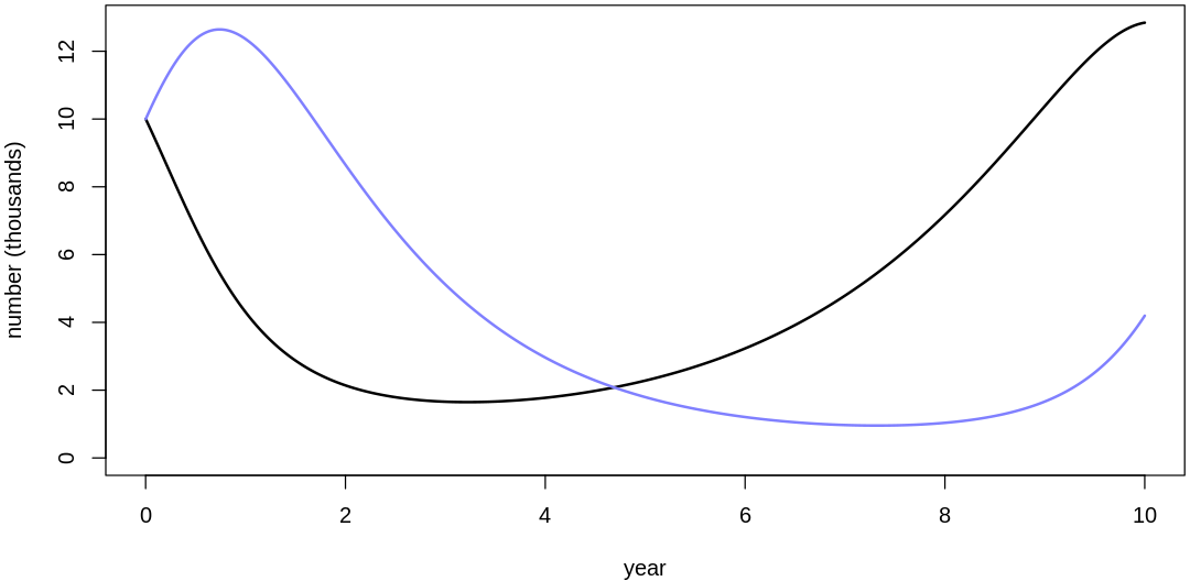
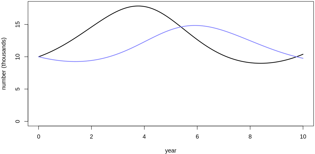
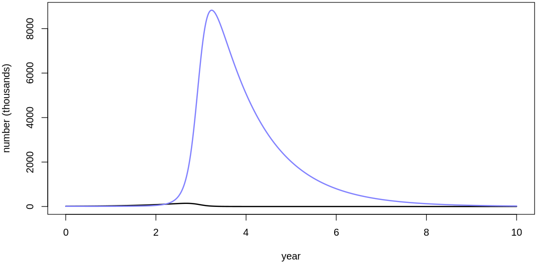
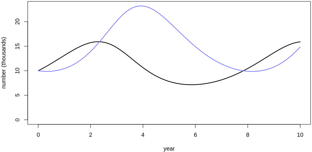
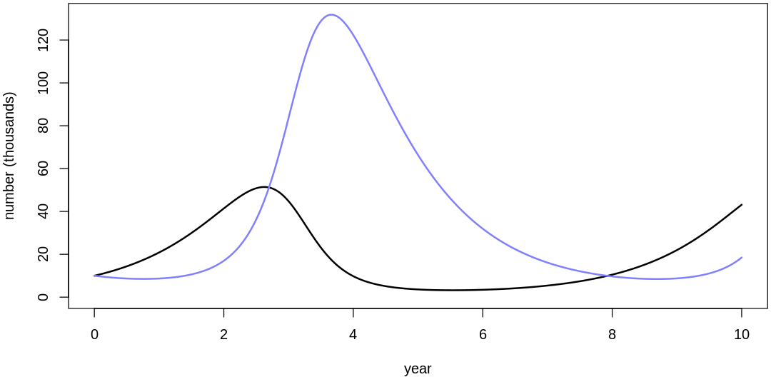
Clearly, these priors produce extreme observations. In some cases populations vary from nearly zero individuals to tens of millions. In any real ecosystem this would not happen; species would go extinct if they hit an extreme population bottleneck.

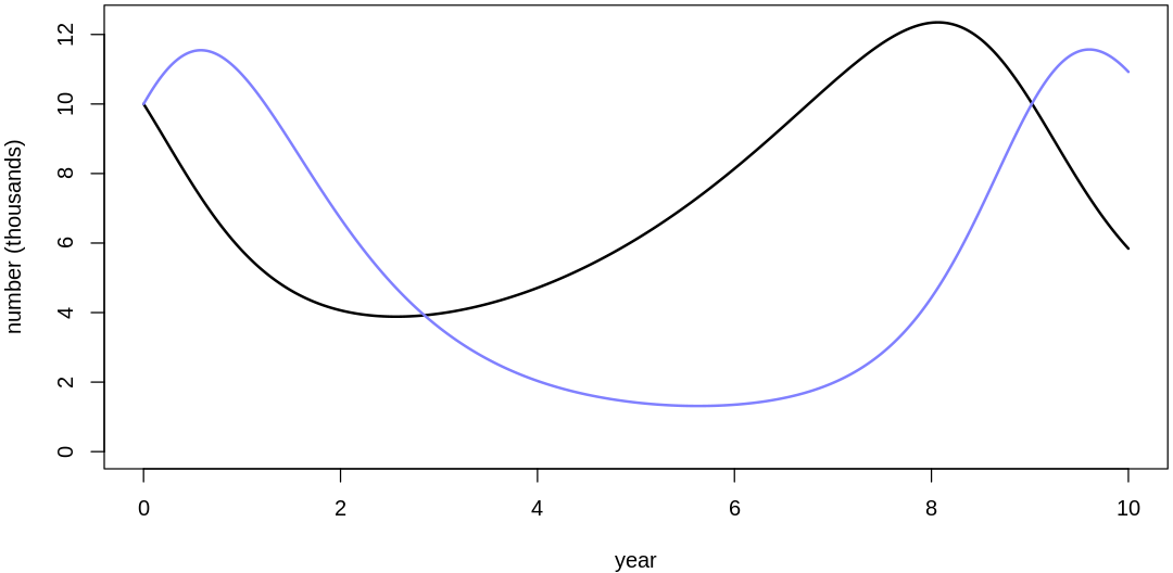
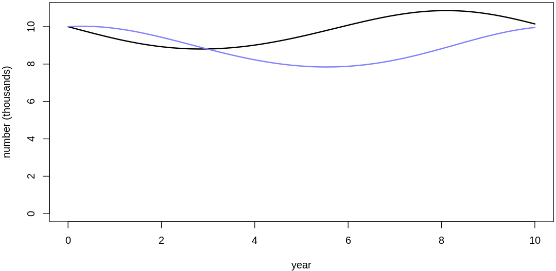
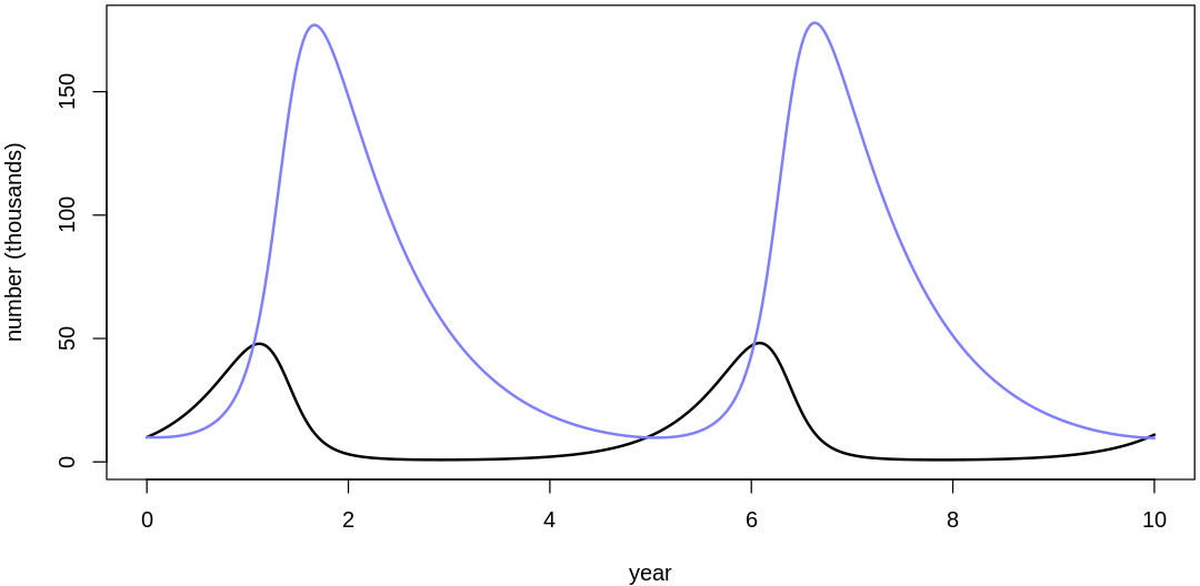
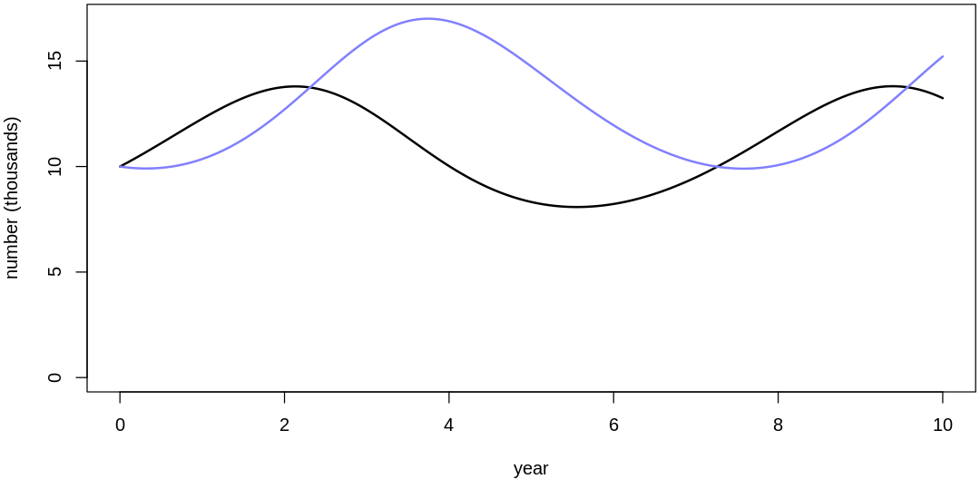
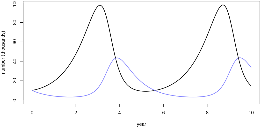
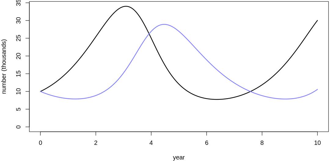
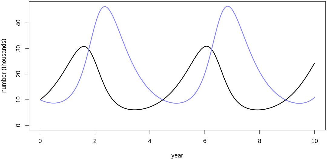
A simple solution is to assume a species’s birth and death rates are not several orders of magnitude off from each other, and to reduce the magnitude of dispersion parameters (standard deviations).

s16m2b <- function() {
  set.seed(7)
  N <- 10
  bH_sim <- abs(rnorm(N, mean=1, sd=0.2))
  bL_sim <- abs(rnorm(N, mean=0.05*bH_sim, sd=0.02*bH_sim))
  mH_sim <- abs(rnorm(N, mean=0.05*bH_sim, sd=0.02*bH_sim))
  mL_sim <- abs(rnorm(N, mean=bH_sim, sd=0.2*bH_sim))
  for (i in 1:length(bH_sim)) {
    theta = list(bH=bH_sim[i], mH=mH_sim[i], bL=bL_sim[i], mL=mL_sim[i])
    pp16m3(theta)
  }
}
s16m2b()

$bH

1.4574494322681

$mH

0.097350345311026

$bL

0.0832782591878165

$mL

1.20360516658157

$bH

0.76064566355553

$mH

0.0487625872778282

$bL

0.0793619924336793

$mL

0.869982476666556

$bH

0.861141497912908

$mH

0.0655494832136692

$bL

0.0823501334749041

$mL

0.88019905489504

$bH

0.91754140977264

$mH

0.0204061903819981

$bL

0.0518231157525117

$mL

0.903142107991628

$bH

0.805865331776103

$mH

0.060809258011534

$bL

0.0708527609060957

$mL

0.738093595070838

$bH

0.810544010954378

$mH

0.0435131274994437

$bL

0.0481087132975566

$mL

0.719418458469278

$bH

1.14962786805811

$mH

0.0747782320573573

$bL

0.0369306290079152

$mL

1.37898171902878

$bH

0.97660895482257

$mH

0.0603885180852695

$bL

0.0428276563531601

$mL

0.760752972486445

$bH

1.03053152525645

$mH

0.0312652424442779

$bL

0.0514271830993257

$mL

1.00120510620173

$bH

1.43799562146588

$mH

0.0639602058993815

$bL

0.100319295478703

$mL

1.52858788026845

16M4. Modify the cylinder height model to use a sphere instead of a cylinder. What choices do you have to make now? Is this a better model, on a predictive basis? Why or why not?

Answer. Fitting the previous model, for reference:

d <- load.d16m1()
m16.1 <- fm16m1(d)

Raw data (following plot):

      mean      sd          5.5%      94.5%     n_eff    Rhat4   
p     0.2441662 0.052323201 0.1751571 0.3376864 547.2458 1.001239
k     5.7650903 2.454602227 2.6396409 9.8224591 553.4296 1.003618
sigma 0.2064420 0.006326218 0.1965793 0.2169334 705.8467 1.008071

A spherical man (or cow) doesn’t seem as helpful for selecting intelligent priors like p. On the other hand, even the cyclinder model required us to pick a prior for k that was based on a fit to maximums in the data rather than introducing more helpful independent information from our experiences. When we select priors based on maximums we’re only easing the fitting process rather than potentially improving the model’s inferences. Still, the process of scaling inputs based on maximums improves our ability to interpret model internals like the priors, which we need to interpret again as the posterior.

The explicitly stated model:

\[ W = kV = k \cdot \frac{4}{3} \pi r^3 \]

Using \(h = 2r\):

\[ W = k \cdot \frac{\pi}{6} h^3 \]

We’ll use a similar equation to the one in the text (based on maximums) to select the prior for k in this scenario:

\[ 1 = k \cdot \frac{\pi}{6} 1^3 \]

Solving for k:

\[ k = \frac{6}{\pi} \]

Fitting the new model:

fmsph <- function(d) {
  msph <- ulam(
    alist(
      w ~ dlnorm(mu, sigma),
      exp(mu) <- 3.141593 * k * h^3,
      k ~ exponential(3.141593 / 6),
      sigma ~ exponential(1)
    ),
    data = d, chains = 4, cores = 4
  )
  display_precis(msph, "msph", ar=4.0)
  vcpp(msph, d)
  return(msph)
}
msph <- fmsph(d)

Raw data (following plot):

      mean      sd          5.5%      94.5%     n_eff    Rhat4   
k     0.3018035 0.002640479 0.2975427 0.3059860 1559.085 1.004879
sigma 0.2066188 0.006074242 0.1971593 0.2163729 1116.351 1.001377

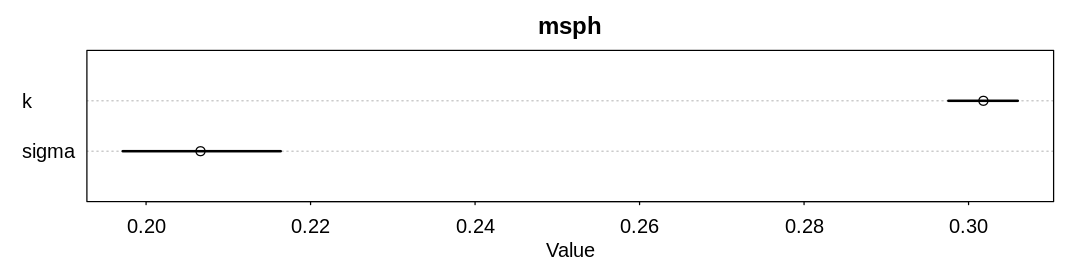
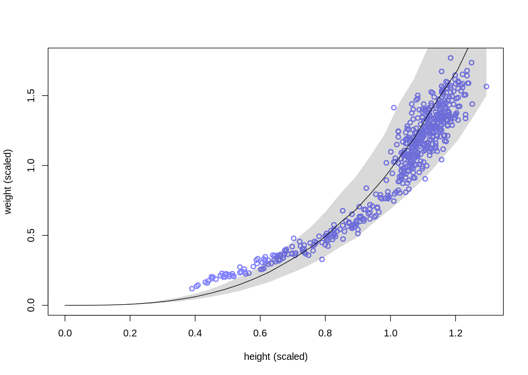
We’ve replaced the k and p parameters, which were previously non-identifiable with respect to one another, with a single parameter. With this change the number of effective samples has improved dramatically, but the posterior predictions are essentially the same.

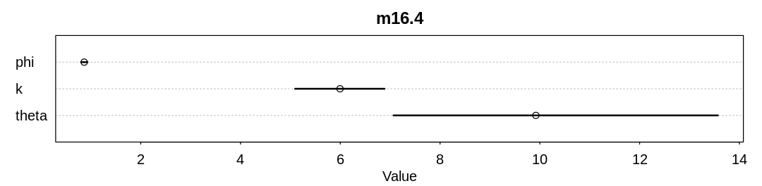
16H1. Modify the Panda nut opening model so that male and female chimpanzees have different maximum adult body mass. The sex variable in data(Panda_nuts) provides the information you need. Be sure to incorporate the fact that you know, prior to seeing the data, that males are on average larger than females at maturity.

Answer. First, let’s reproduce results from the chapter:

load.panda.nut.data <- function() {
  data(Panda_nuts)
  Panda_nuts$sex_int <- as.integer(ifelse(Panda_nuts$sex == 'm', 2, 1))
  display_markdown("The `Panda_nuts` data.frame, with the new predictor as an additional column:")
  display(Panda_nuts)
  return(Panda_nuts)
}
fit.panda.nut.example <- function() {
  data(Panda_nuts)
  dat_list <- list(
    n = as.integer(Panda_nuts$nuts_opened),
    age = Panda_nuts$age / max(Panda_nuts$age),
    seconds = Panda_nuts$seconds
  )
  m16.4 <- ulam(
    alist(
      n ~ poisson(lambda),
      lambda <- seconds * phi * (1 - exp(-k * age))^theta,
      phi ~ lognormal(log(1), 0.1),
      k ~ lognormal(log(2), 0.25),
      theta ~ lognormal(log(5), 0.25)
    ),
    data = dat_list, chains = 4
  )
  display_precis(m16.4, "m16.4", ar=4.0)
}
fit.panda.nut.example()
d <- load.panda.nut.data()

SAMPLING FOR MODEL '36b13a4a3d6bae56fb4ea916b4826328' NOW (CHAIN 1).
Chain 1: 
Chain 1: Gradient evaluation took 3.6e-05 seconds
Chain 1: 1000 transitions using 10 leapfrog steps per transition would take 0.36 seconds.
Chain 1: Adjust your expectations accordingly!
Chain 1: 
Chain 1: 
Chain 1: Iteration:   1 / 1000 [  0%]  (Warmup)
Chain 1: Iteration: 100 / 1000 [ 10%]  (Warmup)
Chain 1: Iteration: 200 / 1000 [ 20%]  (Warmup)
Chain 1: Iteration: 300 / 1000 [ 30%]  (Warmup)
Chain 1: Iteration: 400 / 1000 [ 40%]  (Warmup)
Chain 1: Iteration: 500 / 1000 [ 50%]  (Warmup)
Chain 1: Iteration: 501 / 1000 [ 50%]  (Sampling)
Chain 1: Iteration: 600 / 1000 [ 60%]  (Sampling)
Chain 1: Iteration: 700 / 1000 [ 70%]  (Sampling)
Chain 1: Iteration: 800 / 1000 [ 80%]  (Sampling)
Chain 1: Iteration: 900 / 1000 [ 90%]  (Sampling)
Chain 1: Iteration: 1000 / 1000 [100%]  (Sampling)
Chain 1: 
Chain 1:  Elapsed Time: 0.271681 seconds (Warm-up)
Chain 1:                0.258174 seconds (Sampling)
Chain 1:                0.529855 seconds (Total)
Chain 1: 

SAMPLING FOR MODEL '36b13a4a3d6bae56fb4ea916b4826328' NOW (CHAIN 2).
Chain 2: 
Chain 2: Gradient evaluation took 2.6e-05 seconds
Chain 2: 1000 transitions using 10 leapfrog steps per transition would take 0.26 seconds.
Chain 2: Adjust your expectations accordingly!
Chain 2: 
Chain 2: 
Chain 2: Iteration:   1 / 1000 [  0%]  (Warmup)
Chain 2: Iteration: 100 / 1000 [ 10%]  (Warmup)
Chain 2: Iteration: 200 / 1000 [ 20%]  (Warmup)
Chain 2: Iteration: 300 / 1000 [ 30%]  (Warmup)
Chain 2: Iteration: 400 / 1000 [ 40%]  (Warmup)
Chain 2: Iteration: 500 / 1000 [ 50%]  (Warmup)
Chain 2: Iteration: 501 / 1000 [ 50%]  (Sampling)
Chain 2: Iteration: 600 / 1000 [ 60%]  (Sampling)
Chain 2: Iteration: 700 / 1000 [ 70%]  (Sampling)
Chain 2: Iteration: 800 / 1000 [ 80%]  (Sampling)
Chain 2: Iteration: 900 / 1000 [ 90%]  (Sampling)
Chain 2: Iteration: 1000 / 1000 [100%]  (Sampling)
Chain 2: 
Chain 2:  Elapsed Time: 0.2623 seconds (Warm-up)
Chain 2:                0.244804 seconds (Sampling)
Chain 2:                0.507104 seconds (Total)
Chain 2: 

SAMPLING FOR MODEL '36b13a4a3d6bae56fb4ea916b4826328' NOW (CHAIN 3).
Chain 3: 
Chain 3: Gradient evaluation took 2.5e-05 seconds
Chain 3: 1000 transitions using 10 leapfrog steps per transition would take 0.25 seconds.
Chain 3: Adjust your expectations accordingly!
Chain 3: 
Chain 3: 
Chain 3: Iteration:   1 / 1000 [  0%]  (Warmup)
Chain 3: Iteration: 100 / 1000 [ 10%]  (Warmup)
Chain 3: Iteration: 200 / 1000 [ 20%]  (Warmup)
Chain 3: Iteration: 300 / 1000 [ 30%]  (Warmup)
Chain 3: Iteration: 400 / 1000 [ 40%]  (Warmup)
Chain 3: Iteration: 500 / 1000 [ 50%]  (Warmup)
Chain 3: Iteration: 501 / 1000 [ 50%]  (Sampling)
Chain 3: Iteration: 600 / 1000 [ 60%]  (Sampling)
Chain 3: Iteration: 700 / 1000 [ 70%]  (Sampling)
Chain 3: Iteration: 800 / 1000 [ 80%]  (Sampling)
Chain 3: Iteration: 900 / 1000 [ 90%]  (Sampling)
Chain 3: Iteration: 1000 / 1000 [100%]  (Sampling)
Chain 3: 
Chain 3:  Elapsed Time: 0.230661 seconds (Warm-up)
Chain 3:                0.209069 seconds (Sampling)
Chain 3:                0.43973 seconds (Total)
Chain 3: 

SAMPLING FOR MODEL '36b13a4a3d6bae56fb4ea916b4826328' NOW (CHAIN 4).
Chain 4: 
Chain 4: Gradient evaluation took 2.4e-05 seconds
Chain 4: 1000 transitions using 10 leapfrog steps per transition would take 0.24 seconds.
Chain 4: Adjust your expectations accordingly!
Chain 4: 
Chain 4: 
Chain 4: Iteration:   1 / 1000 [  0%]  (Warmup)
Chain 4: Iteration: 100 / 1000 [ 10%]  (Warmup)
Chain 4: Iteration: 200 / 1000 [ 20%]  (Warmup)
Chain 4: Iteration: 300 / 1000 [ 30%]  (Warmup)
Chain 4: Iteration: 400 / 1000 [ 40%]  (Warmup)
Chain 4: Iteration: 500 / 1000 [ 50%]  (Warmup)
Chain 4: Iteration: 501 / 1000 [ 50%]  (Sampling)
Chain 4: Iteration: 600 / 1000 [ 60%]  (Sampling)
Chain 4: Iteration: 700 / 1000 [ 70%]  (Sampling)
Chain 4: Iteration: 800 / 1000 [ 80%]  (Sampling)
Chain 4: Iteration: 900 / 1000 [ 90%]  (Sampling)
Chain 4: Iteration: 1000 / 1000 [100%]  (Sampling)
Chain 4: 
Chain 4:  Elapsed Time: 0.220774 seconds (Warm-up)
Chain 4:                0.27371 seconds (Sampling)
Chain 4:                0.494484 seconds (Total)
Chain 4: 

Raw data (following plot):

      mean      sd         5.5%      94.5%      n_eff    Rhat4   
phi   0.8664242 0.03898402 0.8055174  0.9321739 714.5807 1.010406
k     5.9948804 0.56300779 5.0935368  6.8870043 629.5435 1.012974
theta 9.9201277 2.01458253 7.0656324 13.5690439 684.8465 1.010622

The Panda_nuts data.frame, with the new predictor as an additional column:

A data.frame: 84 × 8

chimpanzee	age	sex	hammer	nuts_opened	seconds	help	sex_int
<int>	<int>	<fct>	<fct>	<int>	<dbl>	<fct>	<int>
11	3	m	G	0	61.0	N	2
11	3	m	G	0	37.0	N	2
18	4	f	wood	0	20.0	N	1
18	4	f	G	0	14.0	y	1
18	4	f	L	0	13.0	N	1
11	4	m	Q	0	24.0	N	2
11	4	m	Q	0	30.5	N	2
17	5	f	wood	0	135.0	N	1
7	5	m	G	3	24.0	N	2
1	5	m	L	0	13.0	N	2
22	5	m	wood	0	34.0	N	2
9	6	m	G	58	66.5	N	2
9	6	m	G	4	5.0	N	2
9	6	m	G	21	24.0	N	2
9	6	m	G	9	20.0	N	2
9	6	m	G	2	6.0	N	2
9	6	m	G	30	42.0	N	2
9	6	m	G	19	43.0	N	2
9	6	m	G	13	26.5	N	2
9	6	m	G	6	14.0	N	2
15	6	m	G	11	27.0	N	2
7	6	m	G	1	12.0	y	2
9	6	m	G	2	17.0	N	2
1	6	m	L	0	4.0	N	2
7	6	m	G	1	17.0	N	2
13	6	m	wood	0	17.0	N	2
13	6	m	G	0	15.0	N	2
7	6	m	G	0	12.0	y	2
13	6	m	G	0	23.0	y	2
7	6	m	wood	0	47.0	N	2
⋮	⋮	⋮	⋮	⋮	⋮	⋮	⋮
9	8	m	L	0	11.0	N	2
4	9	f	G	1	4.5	N	1
4	9	f	wood	0	17.0	N	1
9	9	m	G	30	47.0	N	2
9	9	m	G	13	24.0	N	2
9	9	m	G	15	34.5	N	2
4	10	f	G	0	2.5	N	1
8	11	f	G	4	13.0	N	1
14	12	f	G	10	10.0	N	1
21	13	f	G	5	13.0	N	1
12	13	m	G	51	43.0	N	2
5	13	m	G	3	6.0	N	2
5	13	m	G	4	6.5	N	2
20	14	m	G	50	50.0	N	2
20	14	m	G	36	48.0	N	2
20	14	m	G	6	14.5	N	2
20	14	m	G	3	8.5	N	2
20	14	m	G	4	15.0	N	2
20	14	m	G	7	17.0	N	2
20	15	m	G	41	56.5	N	2
10	15	m	G	27	33.0	N	2
6	15	m	G	30	36.0	N	2
20	15	m	G	17	42.0	N	2
20	15	m	G	14	23.0	N	2
6	15	m	G	16	20.0	N	2
10	15	m	G	7	12.0	N	2
10	15	m	G	5	12.5	N	2
6	15	m	G	8	13.0	N	2
6	16	m	G	24	20.0	N	2
6	16	m	G	25	36.0	N	2

To include the sex predictor, let’s reconsider the following equation from the text:

\[ \lambda = \alpha S_t^{\theta} = \alpha (\beta M_{max}(1 - exp(-k t)))^{\theta} \]

We’d like to make \(M_{max}\) depend on sex:

\[ \lambda = \alpha (\beta M_{max,sex}(1 - exp(-k t)))^{\theta} \]

We can still scale the \(M\) predictors, but with the new understanding that we are now scaling by the maximum male body size rather than just a general maximum. We can then expect that \(M_{max,male}\) to be one after scaling. We can treat \(M_{max,female}\) as a parameter we expect to be less than one. For our prior we can use information from Chimpanzee: a male chimp averages 55 kg at maturity and a female chimp averages about 40 kg.

Merging several non-identifiable parameters similarly to the text, we have:

\[ \lambda = \phi_{sex} (1 - exp(-k t))^{\theta} \]

We can use the same priors from the text, other than for \(\phi_{sex}\). Because we continued to scale the \(M\) predictors, however, we can reuse the \(\phi_{male}\) prior and effectively only add one new parameter for the female sex:

\[\begin{split} \begin{align} \phi_{male} & \sim LogNormal \left( log(1), 0.1 \right) \\ \phi_{female} & \sim LogNormal \left( log(\frac{40}{55}), 0.1) \right) \end{align} \end{split}\]

For simplicity, we’ll set the same prior and learn the minor difference from the data:

fit.panda.nut.example.with.sex.predictor <- function(d) {
  dat_list <- list(
    n = as.integer(d$nuts_opened),
    age = d$age / max(d$age),
    seconds = d$seconds,
    sex = d$sex_int
  )
  m.with.sex.predictor <- ulam(
    alist(
      n ~ poisson(lambda),
      lambda <- seconds * phi[sex] * (1 - exp(-k * age))^theta,
      phi[sex] ~ lognormal(log(1), 0.1),
      k ~ lognormal(log(2), 0.25),
      theta ~ lognormal(log(5), 0.25)
    ),
    data = dat_list, chains = 4
  )
  display_precis(m.with.sex.predictor, "m.with.sex.predictor", ar=4.0)
}
fit.panda.nut.example.with.sex.predictor(d)

SAMPLING FOR MODEL 'f1e2c316191c1b18560afabfd7eab50b' NOW (CHAIN 1).
Chain 1: 
Chain 1: Gradient evaluation took 2.8e-05 seconds
Chain 1: 1000 transitions using 10 leapfrog steps per transition would take 0.28 seconds.
Chain 1: Adjust your expectations accordingly!
Chain 1: 
Chain 1: 
Chain 1: Iteration:   1 / 1000 [  0%]  (Warmup)
Chain 1: Iteration: 100 / 1000 [ 10%]  (Warmup)
Chain 1: Iteration: 200 / 1000 [ 20%]  (Warmup)
Chain 1: Iteration: 300 / 1000 [ 30%]  (Warmup)
Chain 1: Iteration: 400 / 1000 [ 40%]  (Warmup)
Chain 1: Iteration: 500 / 1000 [ 50%]  (Warmup)
Chain 1: Iteration: 501 / 1000 [ 50%]  (Sampling)
Chain 1: Iteration: 600 / 1000 [ 60%]  (Sampling)
Chain 1: Iteration: 700 / 1000 [ 70%]  (Sampling)
Chain 1: Iteration: 800 / 1000 [ 80%]  (Sampling)
Chain 1: Iteration: 900 / 1000 [ 90%]  (Sampling)
Chain 1: Iteration: 1000 / 1000 [100%]  (Sampling)
Chain 1: 
Chain 1:  Elapsed Time: 0.373572 seconds (Warm-up)
Chain 1:                0.315043 seconds (Sampling)
Chain 1:                0.688615 seconds (Total)
Chain 1: 

SAMPLING FOR MODEL 'f1e2c316191c1b18560afabfd7eab50b' NOW (CHAIN 2).
Chain 2: 
Chain 2: Gradient evaluation took 2.7e-05 seconds
Chain 2: 1000 transitions using 10 leapfrog steps per transition would take 0.27 seconds.
Chain 2: Adjust your expectations accordingly!
Chain 2: 
Chain 2: 
Chain 2: Iteration:   1 / 1000 [  0%]  (Warmup)
Chain 2: Iteration: 100 / 1000 [ 10%]  (Warmup)
Chain 2: Iteration: 200 / 1000 [ 20%]  (Warmup)
Chain 2: Iteration: 300 / 1000 [ 30%]  (Warmup)
Chain 2: Iteration: 400 / 1000 [ 40%]  (Warmup)
Chain 2: Iteration: 500 / 1000 [ 50%]  (Warmup)
Chain 2: Iteration: 501 / 1000 [ 50%]  (Sampling)
Chain 2: Iteration: 600 / 1000 [ 60%]  (Sampling)
Chain 2: Iteration: 700 / 1000 [ 70%]  (Sampling)
Chain 2: Iteration: 800 / 1000 [ 80%]  (Sampling)
Chain 2: Iteration: 900 / 1000 [ 90%]  (Sampling)
Chain 2: Iteration: 1000 / 1000 [100%]  (Sampling)
Chain 2: 
Chain 2:  Elapsed Time: 0.357138 seconds (Warm-up)
Chain 2:                0.308105 seconds (Sampling)
Chain 2:                0.665243 seconds (Total)
Chain 2: 

SAMPLING FOR MODEL 'f1e2c316191c1b18560afabfd7eab50b' NOW (CHAIN 3).
Chain 3: 
Chain 3: Gradient evaluation took 2.7e-05 seconds
Chain 3: 1000 transitions using 10 leapfrog steps per transition would take 0.27 seconds.
Chain 3: Adjust your expectations accordingly!
Chain 3: 
Chain 3: 
Chain 3: Iteration:   1 / 1000 [  0%]  (Warmup)
Chain 3: Iteration: 100 / 1000 [ 10%]  (Warmup)
Chain 3: Iteration: 200 / 1000 [ 20%]  (Warmup)
Chain 3: Iteration: 300 / 1000 [ 30%]  (Warmup)
Chain 3: Iteration: 400 / 1000 [ 40%]  (Warmup)
Chain 3: Iteration: 500 / 1000 [ 50%]  (Warmup)
Chain 3: Iteration: 501 / 1000 [ 50%]  (Sampling)
Chain 3: Iteration: 600 / 1000 [ 60%]  (Sampling)
Chain 3: Iteration: 700 / 1000 [ 70%]  (Sampling)
Chain 3: Iteration: 800 / 1000 [ 80%]  (Sampling)
Chain 3: Iteration: 900 / 1000 [ 90%]  (Sampling)
Chain 3: Iteration: 1000 / 1000 [100%]  (Sampling)
Chain 3: 
Chain 3:  Elapsed Time: 0.324024 seconds (Warm-up)
Chain 3:                0.364045 seconds (Sampling)
Chain 3:                0.688069 seconds (Total)
Chain 3: 

SAMPLING FOR MODEL 'f1e2c316191c1b18560afabfd7eab50b' NOW (CHAIN 4).
Chain 4: 
Chain 4: Gradient evaluation took 3.3e-05 seconds
Chain 4: 1000 transitions using 10 leapfrog steps per transition would take 0.33 seconds.
Chain 4: Adjust your expectations accordingly!
Chain 4: 
Chain 4: 
Chain 4: Iteration:   1 / 1000 [  0%]  (Warmup)
Chain 4: Iteration: 100 / 1000 [ 10%]  (Warmup)
Chain 4: Iteration: 200 / 1000 [ 20%]  (Warmup)
Chain 4: Iteration: 300 / 1000 [ 30%]  (Warmup)
Chain 4: Iteration: 400 / 1000 [ 40%]  (Warmup)
Chain 4: Iteration: 500 / 1000 [ 50%]  (Warmup)
Chain 4: Iteration: 501 / 1000 [ 50%]  (Sampling)
Chain 4: Iteration: 600 / 1000 [ 60%]  (Sampling)
Chain 4: Iteration: 700 / 1000 [ 70%]  (Sampling)
Chain 4: Iteration: 800 / 1000 [ 80%]  (Sampling)
Chain 4: Iteration: 900 / 1000 [ 90%]  (Sampling)
Chain 4: Iteration: 1000 / 1000 [100%]  (Sampling)
Chain 4: 
Chain 4:  Elapsed Time: 0.336466 seconds (Warm-up)
Chain 4:                0.290322 seconds (Sampling)
Chain 4:                0.626788 seconds (Total)
Chain 4: 

Raw data (following plot):

       mean      sd         5.5%      94.5%      n_eff     Rhat4    
phi[1] 0.5972116 0.04914280 0.5210917  0.6760412 1084.1686 1.0007090
phi[2] 0.9998319 0.05379617 0.9201770  1.0921748  578.0931 0.9991132
k      5.1443123 0.62010644 4.2020044  6.1535347  416.2453 1.0003809
theta  7.5389058 1.70372685 5.1940160 10.5915365  460.5012 1.0009579

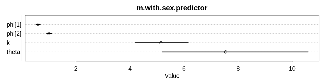
The new model learns significantly different \(\phi\) parameters.

16H2. Now return to the Panda nut model and try to incorporate individual differences. There are two parameters, \(\phi\) and \(k\), which plausibly vary by individual. Pick one of these, allow it to vary by individual, and use partial pooling to avoid overfitting. The variable chimpanzee in data(Panda_nuts) tells you which observations belong to which individuals.

Answer. Pick the \(\phi\) parameter to vary by individual:

fit.panda.nut.example.with.individual.differences <- function() {
  data(Panda_nuts)
  dat_list <- list(
    n = as.integer(Panda_nuts$nuts_opened),
    age = Panda_nuts$age / max(Panda_nuts$age),
    chimp = Panda_nuts$chimpanzee,
    seconds = Panda_nuts$seconds
  )
  m.with.individual.phi <- ulam(
    alist(
      n ~ poisson(lambda),
      lambda <- seconds * phi[chimp] * (1 - exp(-k * age))^theta,
      phi[chimp] ~ lognormal(log(phi_bar), 0.1),
      phi_bar ~ lognormal(log(1), 0.1),
      k ~ lognormal(log(2), 0.25),
      theta ~ lognormal(log(5), 0.25)
    ),
    data = dat_list, chains = 4
  )
  display_precis(m.with.individual.phi, "m.with.individual.phi", ar=1.5)
}
fit.panda.nut.example.with.individual.differences()

SAMPLING FOR MODEL '7fe65127e52ef2f8367f68333fafac3e' NOW (CHAIN 1).
Chain 1: 
Chain 1: Gradient evaluation took 3.2e-05 seconds
Chain 1: 1000 transitions using 10 leapfrog steps per transition would take 0.32 seconds.
Chain 1: Adjust your expectations accordingly!
Chain 1: 
Chain 1: 
Chain 1: Iteration:   1 / 1000 [  0%]  (Warmup)
Chain 1: Iteration: 100 / 1000 [ 10%]  (Warmup)
Chain 1: Iteration: 200 / 1000 [ 20%]  (Warmup)
Chain 1: Iteration: 300 / 1000 [ 30%]  (Warmup)
Chain 1: Iteration: 400 / 1000 [ 40%]  (Warmup)
Chain 1: Iteration: 500 / 1000 [ 50%]  (Warmup)
Chain 1: Iteration: 501 / 1000 [ 50%]  (Sampling)
Chain 1: Iteration: 600 / 1000 [ 60%]  (Sampling)
Chain 1: Iteration: 700 / 1000 [ 70%]  (Sampling)
Chain 1: Iteration: 800 / 1000 [ 80%]  (Sampling)
Chain 1: Iteration: 900 / 1000 [ 90%]  (Sampling)
Chain 1: Iteration: 1000 / 1000 [100%]  (Sampling)
Chain 1: 
Chain 1:  Elapsed Time: 0.620707 seconds (Warm-up)
Chain 1:                0.46885 seconds (Sampling)
Chain 1:                1.08956 seconds (Total)
Chain 1: 

SAMPLING FOR MODEL '7fe65127e52ef2f8367f68333fafac3e' NOW (CHAIN 2).
Chain 2: 
Chain 2: Gradient evaluation took 2.8e-05 seconds
Chain 2: 1000 transitions using 10 leapfrog steps per transition would take 0.28 seconds.
Chain 2: Adjust your expectations accordingly!
Chain 2: 
Chain 2: 
Chain 2: Iteration:   1 / 1000 [  0%]  (Warmup)
Chain 2: Iteration: 100 / 1000 [ 10%]  (Warmup)
Chain 2: Iteration: 200 / 1000 [ 20%]  (Warmup)
Chain 2: Iteration: 300 / 1000 [ 30%]  (Warmup)
Chain 2: Iteration: 400 / 1000 [ 40%]  (Warmup)
Chain 2: Iteration: 500 / 1000 [ 50%]  (Warmup)
Chain 2: Iteration: 501 / 1000 [ 50%]  (Sampling)
Chain 2: Iteration: 600 / 1000 [ 60%]  (Sampling)
Chain 2: Iteration: 700 / 1000 [ 70%]  (Sampling)
Chain 2: Iteration: 800 / 1000 [ 80%]  (Sampling)
Chain 2: Iteration: 900 / 1000 [ 90%]  (Sampling)
Chain 2: Iteration: 1000 / 1000 [100%]  (Sampling)
Chain 2: 
Chain 2:  Elapsed Time: 0.53282 seconds (Warm-up)
Chain 2:                0.520665 seconds (Sampling)
Chain 2:                1.05349 seconds (Total)
Chain 2: 

SAMPLING FOR MODEL '7fe65127e52ef2f8367f68333fafac3e' NOW (CHAIN 3).
Chain 3: 
Chain 3: Gradient evaluation took 2.8e-05 seconds
Chain 3: 1000 transitions using 10 leapfrog steps per transition would take 0.28 seconds.
Chain 3: Adjust your expectations accordingly!
Chain 3: 
Chain 3: 
Chain 3: Iteration:   1 / 1000 [  0%]  (Warmup)
Chain 3: Iteration: 100 / 1000 [ 10%]  (Warmup)
Chain 3: Iteration: 200 / 1000 [ 20%]  (Warmup)
Chain 3: Iteration: 300 / 1000 [ 30%]  (Warmup)
Chain 3: Iteration: 400 / 1000 [ 40%]  (Warmup)
Chain 3: Iteration: 500 / 1000 [ 50%]  (Warmup)
Chain 3: Iteration: 501 / 1000 [ 50%]  (Sampling)
Chain 3: Iteration: 600 / 1000 [ 60%]  (Sampling)
Chain 3: Iteration: 700 / 1000 [ 70%]  (Sampling)
Chain 3: Iteration: 800 / 1000 [ 80%]  (Sampling)
Chain 3: Iteration: 900 / 1000 [ 90%]  (Sampling)
Chain 3: Iteration: 1000 / 1000 [100%]  (Sampling)
Chain 3: 
Chain 3:  Elapsed Time: 0.62722 seconds (Warm-up)
Chain 3:                0.432308 seconds (Sampling)
Chain 3:                1.05953 seconds (Total)
Chain 3: 

SAMPLING FOR MODEL '7fe65127e52ef2f8367f68333fafac3e' NOW (CHAIN 4).
Chain 4: 
Chain 4: Gradient evaluation took 2.7e-05 seconds
Chain 4: 1000 transitions using 10 leapfrog steps per transition would take 0.27 seconds.
Chain 4: Adjust your expectations accordingly!
Chain 4: 
Chain 4: 
Chain 4: Iteration:   1 / 1000 [  0%]  (Warmup)
Chain 4: Iteration: 100 / 1000 [ 10%]  (Warmup)
Chain 4: Iteration: 200 / 1000 [ 20%]  (Warmup)
Chain 4: Iteration: 300 / 1000 [ 30%]  (Warmup)
Chain 4: Iteration: 400 / 1000 [ 40%]  (Warmup)
Chain 4: Iteration: 500 / 1000 [ 50%]  (Warmup)
Chain 4: Iteration: 501 / 1000 [ 50%]  (Sampling)
Chain 4: Iteration: 600 / 1000 [ 60%]  (Sampling)
Chain 4: Iteration: 700 / 1000 [ 70%]  (Sampling)
Chain 4: Iteration: 800 / 1000 [ 80%]  (Sampling)
Chain 4: Iteration: 900 / 1000 [ 90%]  (Sampling)
Chain 4: Iteration: 1000 / 1000 [100%]  (Sampling)
Chain 4: 
Chain 4:  Elapsed Time: 0.553959 seconds (Warm-up)
Chain 4:                0.443515 seconds (Sampling)
Chain 4:                0.997474 seconds (Total)
Chain 4: 

Warning message:
“Bulk Effective Samples Size (ESS) is too low, indicating posterior means and medians may be unreliable.
Running the chains for more iterations may help. See
https://mc-stan.org/misc/warnings.html#bulk-ess”

Warning message:
“Tail Effective Samples Size (ESS) is too low, indicating posterior variances and tail quantiles may be unreliable.
Running the chains for more iterations may help. See
https://mc-stan.org/misc/warnings.html#tail-ess”

Raw data (following plot):

        mean      sd         5.5%      94.5%     n_eff    Rhat4   
phi[1]  0.9553298 0.12212570 0.7678728 1.1573779 416.7093 1.005197
phi[2]  0.9327892 0.11401365 0.7608654 1.1247825 433.4090 1.005205
phi[3]  0.8910858 0.10556602 0.7333032 1.0640384 415.3170 1.002631
phi[4]  0.8925237 0.10617508 0.7295207 1.0680879 427.1174 1.004093
phi[5]  0.9597426 0.11676147 0.7889388 1.1503983 420.5202 1.002604
phi[6]  0.9775833 0.08947604 0.8385866 1.1286809 386.2900 1.003889
phi[7]  0.8611309 0.10534897 0.7049017 1.0405510 447.7295 1.003798
phi[8]  0.9440603 0.11125720 0.7753973 1.1276879 398.3424 1.002574
phi[9]  1.9607894 0.19906902 1.6728647 2.3047344 270.5416 1.006690
phi[10] 0.9281008 0.09608783 0.7803962 1.0832118 415.5111 1.002687
phi[11] 0.9305691 0.11348198 0.7615222 1.1203311 475.9042 1.001189
phi[12] 1.1334487 0.12670496 0.9423372 1.3508605 446.2032 1.007387
phi[13] 0.8867634 0.10839310 0.7271997 1.0624630 398.6809 1.001864
phi[14] 1.0106827 0.12545045 0.8258410 1.2216117 432.3781 1.004352
phi[15] 1.0351239 0.12842910 0.8407328 1.2582050 444.5947 1.002829
phi[16] 0.8595452 0.10097075 0.7081932 1.0323313 424.4016 1.003874
phi[17] 0.8485815 0.10421533 0.6935252 1.0250191 441.2525 1.004045
phi[18] 0.9523250 0.11178543 0.7822926 1.1393024 440.3078 1.002757
phi[19] 1.1635026 0.12727116 0.9789523 1.3887908 345.8941 1.003416
phi[20] 0.8639027 0.07046997 0.7562107 0.9785163 364.3745 1.004556
phi[21] 0.9403173 0.11015485 0.7734515 1.1244005 386.8617 1.002809
phi[22] 0.9399306 0.11493340 0.7700160 1.1382278 422.0380 1.006429
phi_bar 0.9739713 0.07182947 0.8583567 1.0944214 203.6917 1.008876
k       3.6021006 0.43971265 2.8939478 4.3054850 285.3794 1.006284
theta   5.4003882 0.92929170 4.0694794 6.9970231 439.1491 1.003484

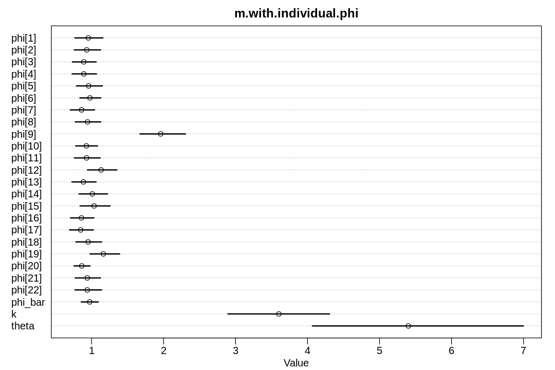
There’s a lot of individual variation; the 9th chimpanzee is a standout even with regularization.

16H3. The chapter asserts that a typical, geocentric time series model might be one that uses lag variables. Here you’ll fit such a model and compare it to the ODE model in the chapter. An autoregressive time series uses earlier values of the state variables to predict new values of the same variables. These earlier values are called lag variables. You can construct the lag variables here with:

R code 16.21

data(Lynx_Hare)
dat_ar1 <- list(
 L = Lynx_Hare$Lynx[2:21],
 L_lag1 = Lynx_Hare$Lynx[1:20],
 H = Lynx_Hare$Hare[2:21],
 H_lag1 = Lynx_Hare$Hare[1:20] )

Now you can use L_lag1 and H_lag1 as predictors of the outcomes L and H. Like this:

\[\begin{split} \begin{align} L_t \sim LogNormal(log(\mu_{L,t}), \sigma_L) \\ \mu_{L,t} = \alpha_L + \beta_{LL}L_{t-1} + \beta_{LH}H_{t-1} \\ H_t \sim LogNormal(log(\mu_{H,t}), \sigma_H) \\ \mu_{H,t} = \alpha_H + \beta_{HH}H_{t-1} + \beta_{HL}L_{t-1} \end{align} \end{split}\]

where \(L_{t-1}\) and \(H_{t–1}\) are the lag variables. Use ulam() to fit this model. Be careful of the priors of the \(\alpha\) and \(\beta\) parameters. Compare the posterior predictions of the autoregressive model to the ODE model in the chapter. How do the predictions differ? Can you explain why, using the structures of the models?

Answer. First, let’s review the data and reproduce some results from the text.

The entirety of the Lynx_Hare data.frame:

data(Lynx_Hare)
display(Lynx_Hare)

A data.frame: 21 × 3

Year	Lynx	Hare
<int>	<dbl>	<dbl>
1900	4.0	30.0
1901	6.1	47.2
1902	9.8	70.2
1903	35.2	77.4
1904	59.4	36.3
1905	41.7	20.6
1906	19.0	18.1
1907	13.0	21.4
1908	8.3	22.0
1909	9.1	25.4
1910	7.4	27.1
1911	8.0	40.3
1912	12.3	57.0
1913	19.5	76.6
1914	45.7	52.3
1915	51.1	19.5
1916	29.7	11.2
1917	15.8	7.6
1918	9.7	14.6
1919	10.1	16.2
1920	8.6	24.7

The model proposed by the author:

data(Lynx_Hare_model)
cat(Lynx_Hare_model)
flush.console()

functions {
  real[] dpop_dt( real t,                 // time
                real[] pop_init,          // initial state {lynx, hares}
                real[] theta,             // parameters
                real[] x_r, int[] x_i) {  // unused
    real L = pop_init[1];
    real H = pop_init[2];
    real bh = theta[1];
    real mh = theta[2];
    real ml = theta[3];
    real bl = theta[4];
    // differential equations
    real dH_dt = (bh - mh * L) * H;
    real dL_dt = (bl * H - ml) * L;
    return { dL_dt , dH_dt };
  }
}
data {
  int<lower=0> N;              // number of measurement times
  real<lower=0> pelts[N,2];    // measured populations
}
transformed data{
  real times_measured[N-1];    // N-1 because first time is initial state
  for ( i in 2:N ) times_measured[i-1] = i;
}
parameters {
  real<lower=0> theta[4];      // { bh, mh, ml, bl }
  real<lower=0> pop_init[2];   // initial population state
  real<lower=0> sigma[2];      // measurement errors
  real<lower=0,upper=1> p[2];  // trap rate
}
transformed parameters {
  real pop[N, 2];
  pop[1,1] = pop_init[1];
  pop[1,2] = pop_init[2];
  pop[2:N,1:2] = integrate_ode_rk45(
    dpop_dt, pop_init, 0, times_measured, theta,
    rep_array(0.0, 0), rep_array(0, 0),
    1e-5, 1e-3, 5e2);
}
model {
  // priors
  theta[{1,3}] ~ normal( 1 , 0.5 );    // bh,ml
  theta[{2,4}] ~ normal( 0.05, 0.05 ); // mh,bl
  sigma ~ exponential( 1 );
  pop_init ~ lognormal( log(10) , 1 );
  p ~ beta(40,200);
  // observation model
  // connect latent population state to observed pelts
  for ( t in 1:N )
    for ( k in 1:2 )
      pelts[t,k] ~ lognormal( log(pop[t,k]*p[k]) , sigma[k] );
}
generated quantities {
  real pelts_pred[N,2];
  for ( t in 1:N )
    for ( k in 1:2 )
      pelts_pred[t,k] = lognormal_rng( log(pop[t,k]*p[k]) , sigma[k] );
}

plot.lh.posterior <- function(x, hare_pred, lynx_pred, Lynx_Hare, name) {
  pelts <- Lynx_Hare[, 2:3]
  iplot(function() {
    plot(1:21, pelts[, 2],
      main = name, pch = 16, ylim = c(0, 120), xlab = "year",
      ylab = "thousands of pelts", xaxt = "n"
    )
    at <- c(1, 11, 21)
    axis(1, at = at, labels = Lynx_Hare$Year[at])
    points(1:21, pelts[, 1], col = rangi2, pch = 16)
    # 21 time series from posterior
    for (s in 1:21) {
      lines(x, hare_pred[s,], col = col.alpha("black", 0.2), lwd = 2)
      lines(x, lynx_pred[s,], col = col.alpha(rangi2, 0.3), lwd = 2)
    }
    # text labels
    text(17, 90, "Lepus", pos = 2)
    text(19, 50, "Lynx", pos = 2, col = rangi2)
  })
}

reproduce.lh.model <- function() {
  data(Lynx_Hare)
  data(Lynx_Hare_model)
  dat_list <- list(
    N = nrow(Lynx_Hare),
    pelts = Lynx_Hare[, 2:3]
  )
  m16.5 <- stan(
    model_code = Lynx_Hare_model, data = dat_list,
    chains = 4, cores = 4,
    control = list(adapt_delta = 0.95)
  )
  post <- extract.samples(m16.5)
  hare_pred = post$pelts_pred[,,2]
  lynx_pred = post$pelts_pred[,,1]
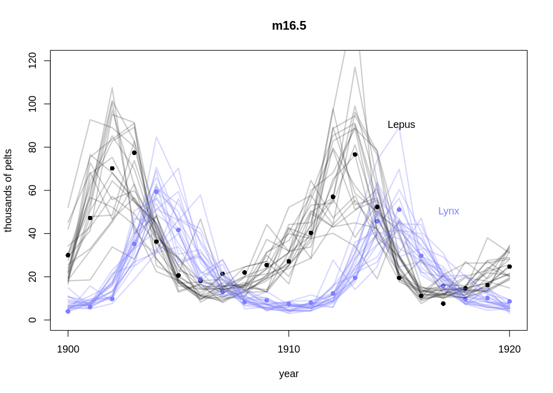
  display_markdown("The posterior predictions from the text:")
  plot.lh.posterior(1:21, hare_pred, lynx_pred, Lynx_Hare, "m16.5")
}
reproduce.lh.model()

The posterior predictions from the text:

Let’s compare the mathematical form of the models side-by-side. The core of the ODE model:

\[\begin{split} \begin{align} H_1 & \sim LogNormal(log(10), 1) \\ L_1 & \sim LogNormal(log(10), 1) \\ H_{T>1} & = H_1 + \int\limits_1^T H_t (b_H - m_H L_t) dt \\ L_{T>1} & = L_1 + \int\limits_1^T L_t (b_L H_t - m_L) dt \end{align} \end{split}\]

The AR model:

\[\begin{split} \begin{align} H_t \sim LogNormal(log(\mu_{H,t}), \sigma_H) \\ \mu_{H,t} = \alpha_H + \beta_{HH}H_{t-1} + \beta_{HL}L_{t-1} \\ L_t \sim LogNormal(log(\mu_{L,t}), \sigma_L) \\ \mu_{L,t} = \alpha_L + \beta_{LL}L_{t-1} + \beta_{LH}H_{t-1} \end{align} \end{split}\]

The ODE model doesn’t have an alpha parameter, which lets Hare and Lynx be created from nothing in the AR model. In the ODE model, the Hare death rate is proportional to the product of the current Hare and Lynx population; in the AR model it is proportional to only the Lynx population. Similarly, Lynx birth rate is proportional to the product of the Hare and Lynx populations rather than only the Lynx population. The ODE model seems to have better assumptions in all these cases.

Because the AR model must always be able to look back one step to make a prediction, one predictive difference we can expect is that it will have one fewer prediction. That is, it will have no prediction for the initial population other than what the data provides. Notice the AR model has no prior for the initial population like the ODE model has.

Critically, the AR model assumes the present population is based on the observed populations from one time step back, and no farther. The ODE model uses the full histories (looking forward and back) to pick model parameters. The ODE model looks forward in the sense that it has parameters for the initial population that will be indirectly updated based on future observations.

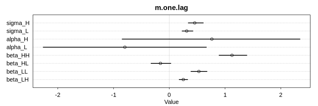
The AR models aren’t designed in a way that we know in a strict sense which parameters should be positive and negative. In the one-lag AR model, we would expect \(\beta_{HH}\) to be positive because hares give birth to more hares, and \(\beta_{HL}\) to be negative because lynx eat hares. It gets harder to make simple prior decisions like this with two lag variables because we can’t strictly interpret the \(\beta\) parameters as birth and death rates.

fit.one.lag.variable <- function() {
  data(Lynx_Hare)
  dat_ar1 <- list(
    L = Lynx_Hare$Lynx[2:21],
    L_lag1 = Lynx_Hare$Lynx[1:20],
    H = Lynx_Hare$Hare[2:21],
    H_lag1 = Lynx_Hare$Hare[1:20]
  )
  m.one.lag <- ulam(
    alist(
      H ~ lognormal(log(mu_H), sigma_H),
      mu_H <- alpha_H + beta_HH * H_lag1 + beta_HL * L_lag1,
      L ~ lognormal(log(mu_L), sigma_L),
      mu_L <- alpha_L + beta_LL * L_lag1 + beta_LH * H_lag1,
      sigma_H ~ dexp(0.5),
      sigma_L ~ dexp(0.5),
      alpha_H ~ dnorm(0, 1),
      alpha_L ~ dnorm(0, 1),
      beta_HH ~ dnorm(0.5, 1),
      beta_HL ~ dnorm(-0.5, 1),
      beta_LL ~ dnorm(0.5, 1),
      beta_LH ~ dnorm(0.5, 1)
    ), data = dat_ar1, cores = 4, chains = 4
  )
  display_markdown("Inferred parameters:")
  iplot(function() {
    plot(precis(m.one.lag), main="m.one.lag")
  }, ar=3)
  display_markdown(r"(Posterior predictions without influence of $\sigma$:)")
  post <- extract.samples(m.one.lag)
  mu_H <- mapply(function(H_l1, L_l1) {
    post$alpha_H + post$beta_HH * H_l1 + post$beta_HL * L_l1
  }, dat_ar1$H_lag1, dat_ar1$L_lag1)
  mu_L <- mapply(function(H_l1, L_l1) {
    post$alpha_L + post$beta_LL * L_l1 + post$beta_LH * H_l1
  }, dat_ar1$H_lag1, dat_ar1$L_lag1)
  plot.lh.posterior(2:21, mu_H, mu_L, Lynx_Hare, "m.one.lag")
}
fit.one.lag.variable()

Inferred parameters:

Posterior predictions without influence of $\sigma$:

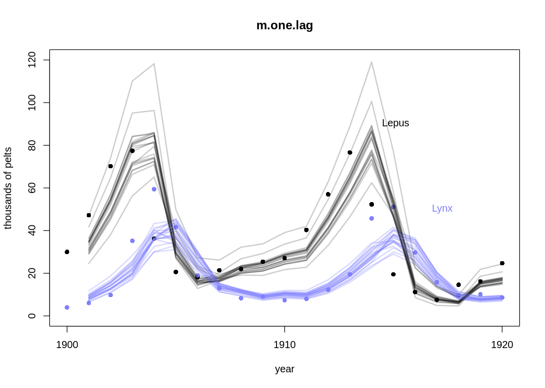
We skip the influence of \(\sigma\) in the previous plot to make it easier to interpret. The AR model generally performs worse than the ODE model, in particular in areas with extreme transitions. Because the AR model is looking at such a more local scale when it updates parameters, it seems to dismiss these extreme cases as outliers in order to fit the majority of the data more closely. That is, it can’t see these cases as the result of a larger trend going back several steps.

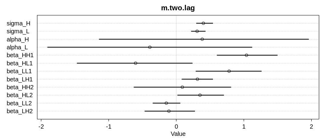
16H4. Adapt the autoregressive model to use a two-step lag variable. This means that \(L_{t–2}\) and \(H_{t–2}\), in addition to \(L_{t–1}\) and \(H_{t–1}\), will appear in the equation for \(\mu\). This implies that prediction depends upon not only what happened just before now, but also on what happened two time steps ago. How does this model perform, compared to the ODE model?

Answer. We’ll extend the previous question’s model in a straightforward way.

fit.two.lag.variable <- function() {
  data(Lynx_Hare)
  dat_ar2 <- list(
    L = Lynx_Hare$Lynx[3:21],
    L_lag1 = Lynx_Hare$Lynx[2:20],
    L_lag2 = Lynx_Hare$Lynx[1:19],
    H = Lynx_Hare$Hare[3:21],
    H_lag1 = Lynx_Hare$Hare[2:20],
    H_lag2 = Lynx_Hare$Hare[1:19]
  )
  m.two.lag <- ulam(
    alist(
      H ~ lognormal(log(mu_H), sigma_H),
      mu_H <- alpha_H + beta_HH1 * H_lag1 + beta_HL1 * L_lag1 + beta_HH2 * H_lag2 + beta_HL2 * L_lag2,
      L ~ lognormal(log(mu_L), sigma_L),
      mu_L <- alpha_L + beta_LL1 * L_lag1 + beta_LH1 * H_lag1 + beta_LL2 * L_lag2 + beta_LH2 * H_lag2,
      sigma_H ~ dexp(0.5),
      sigma_L ~ dexp(0.5),
      alpha_H ~ dnorm(0, 1),
      alpha_L ~ dnorm(0, 1),
      beta_HH1 ~ dnorm(0, 1),
      beta_HL1 ~ dnorm(0, 1),
      beta_LL1 ~ dnorm(0, 1),
      beta_LH1 ~ dnorm(0, 1),
      beta_HH2 ~ dnorm(0, 1),
      beta_HL2 ~ dnorm(0, 1),
      beta_LL2 ~ dnorm(0, 1),
      beta_LH2 ~ dnorm(0, 1)
    ), data = dat_ar2, cores = 4, chains = 4
  )
  display_markdown("Inferred parameters:")
  iplot(function() {
    plot(precis(m.two.lag), main="m.two.lag")
  }, ar=2.4)
  display_markdown(r"(Posterior predictions without influence of $\sigma$:)")
  post <- extract.samples(m.two.lag)
  mu_H <- mapply(function(H_l1, L_l1, H_l2, L_l2) {
    post$alpha_H + post$beta_HH1 * H_l1 + post$beta_HL1 * L_l1 + post$beta_HH2 * H_l2 + post$beta_HL2 * L_l2
  }, dat_ar2$H_lag1, dat_ar2$L_lag1, dat_ar2$H_lag2, dat_ar2$L_lag2)
  mu_L <- mapply(function(H_l1, L_l1, L_l2, H_l2) {
    post$alpha_L + post$beta_LL1 * L_l1 + post$beta_LH1 * H_l1 + post$beta_LL2 * L_l2 + post$beta_LH2 * H_l2
  }, dat_ar2$H_lag1, dat_ar2$L_lag1, dat_ar2$H_lag2, dat_ar2$L_lag2)
  plot.lh.posterior(3:21, mu_H, mu_L, Lynx_Hare, "m.two.lag")
}
fit.two.lag.variable()

Warning message:
“There were 2 divergent transitions after warmup. See
https://mc-stan.org/misc/warnings.html#divergent-transitions-after-warmup
to find out why this is a problem and how to eliminate them.”

Warning message:
“Examine the pairs() plot to diagnose sampling problems
”

Inferred parameters:

Posterior predictions without influence of $\sigma$:

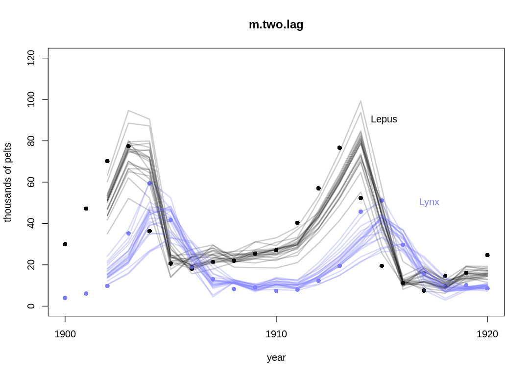
The two-step lag model performs similarly the one-step lag model, with more uncertainty associated with extra parameters that only give the model general flexibility, not the right kind of flexibility for this problem.

16H5. Population dynamic models are typically very difficult to fit to empirical data. The lynx-hare example in the chapter was easy, partly because the data are unusually simple and partly because the chapter did the difficult prior selection for you. Here’s another data set that will impress upon you both how hard the task can be and how badly Lotka-Volterra fits empirical data in general. The data in data(Mites) are numbers of predator and prey mites living on fruit. Model these data using the same Lotka-Volterra ODE system from the chapter. These data are actual counts of individuals, not just their pelts. You will need to adapt the Stan code in data(Lynx_Hare_model). Note that the priors will need to be rescaled, because the outcome variables are on a different scale. Prior predictive simulation will help. Keep in mind as well that the time variable and the birth and death parameters go together. If you rescale the time dimension, that implies you must also rescale the parameters.

Answer. Let’s start by inspecting the data.

load.mites <- function() {
  data(Mites)
  display_markdown("The `Mites` data:")
  display(Mites)
  return(Mites)
}
d <- load.mites()

The Mites data:

A data.frame: 35 × 3

day	prey	predator
<int>	<int>	<int>
16	194	75
23	896	119
29	1443	488
36	851	960
42	308	458
49	264	433
56	194	239
62	204	164
68	214	139
75	348	50
81	498	50
88	572	144
94	1607	154
101	1746	498
108	2100	473
114	1796	711
121	1607	557
127	746	950
133	493	254
140	706	144
147	1801	383
153	1751	80
160	1189	50
166	2005	80
173	1801	50
179	154	119
185	1851	378
192	1493	706
199	493	1209
205	184	313
212	40	85
219	50	50
225	50	50
231	85	50
238	199	50

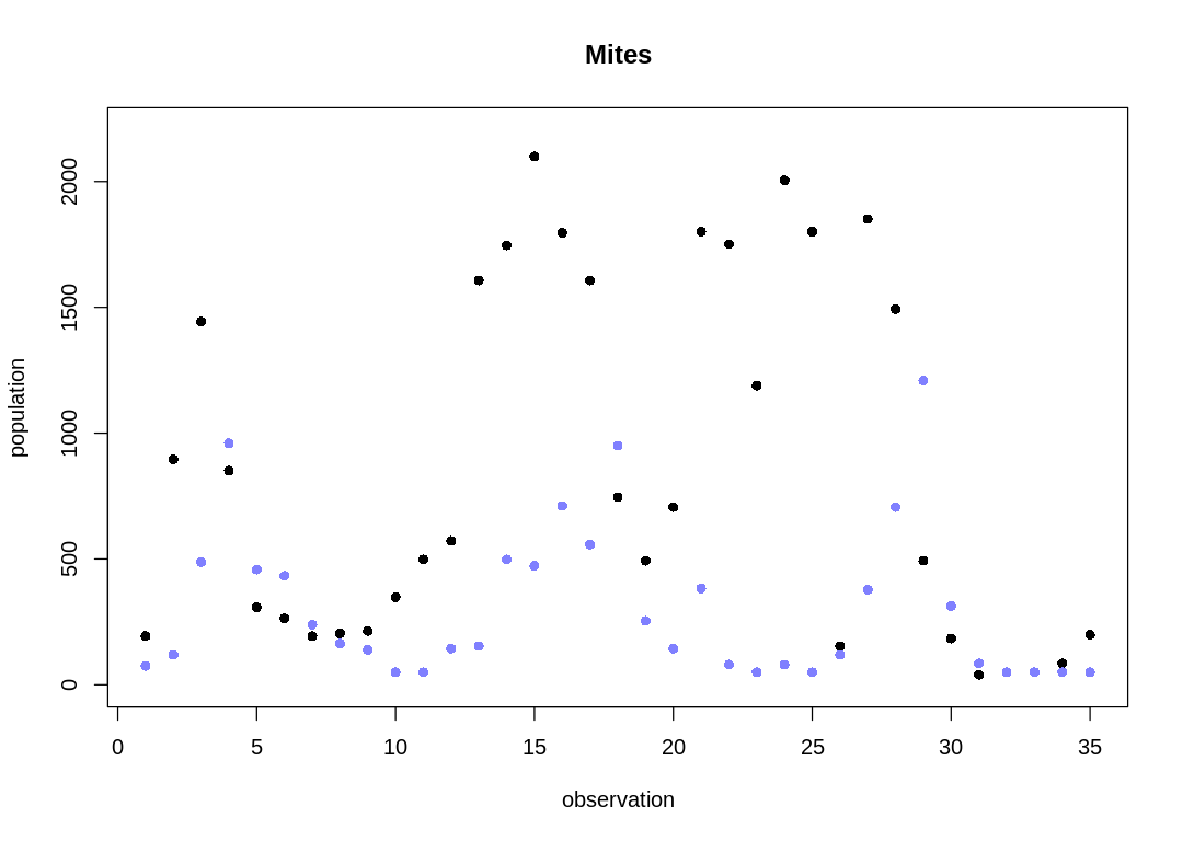
mites.simple.model <- r"(
Notice the observations are usually 6-7 days apart. For modeling simplicity, we'll assume the
observations are evenly spaced. The raw data with this simpler x-axis is:
)"
plot.mites <- function(d) {
  display_markdown("<br/> The `Mites` data on a plot:")
  iplot(function() {
    plot(d$day, d$prey,
      main = "Mites", pch = 16,
      xlim = c(0, max(d$day)*1.05),
      ylim = c(0, max(d$prey)*1.05),
      xlab = "day", ylab = "population"
    )
    points(d$day, d$predator, col = rangi2, pch = 16)
  })
  display_markdown(mites.simple.model)
  iplot(function() {
    N = length(d$day)
    plot(1:N, d$prey,
      main = "Mites", pch = 16,
      ylim = c(0, max(d$prey)*1.05),
      xlab = "observation", ylab = "population"
    )
    points(1:N, d$predator, col = rangi2, pch = 16)
  })
}
plot.mites(d)

The Mites data on a plot:

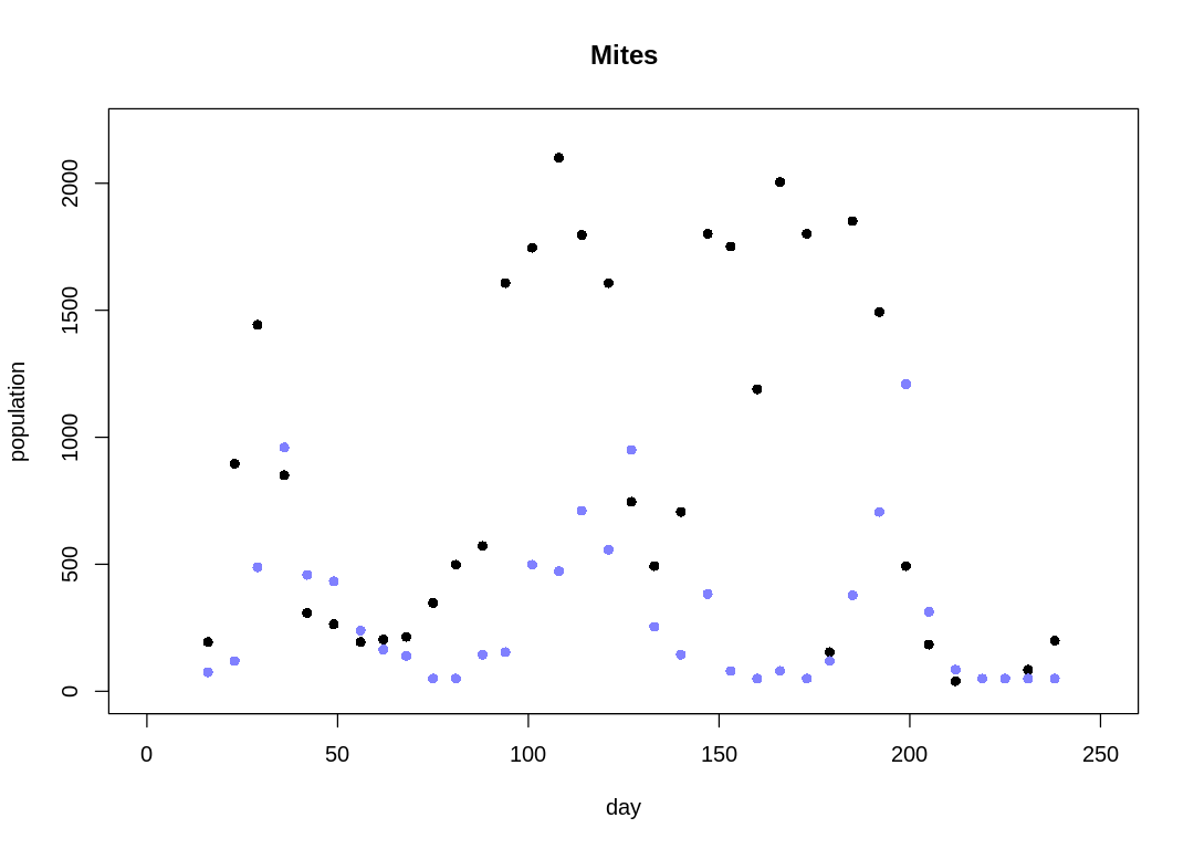
Notice the observations are usually 6-7 days apart. For modeling simplicity, we’ll assume the observations are evenly spaced. The raw data with this simpler x-axis is:

The cyclical trend is less clear than in the Lynx-Hare data (compare to Figure 16.6).

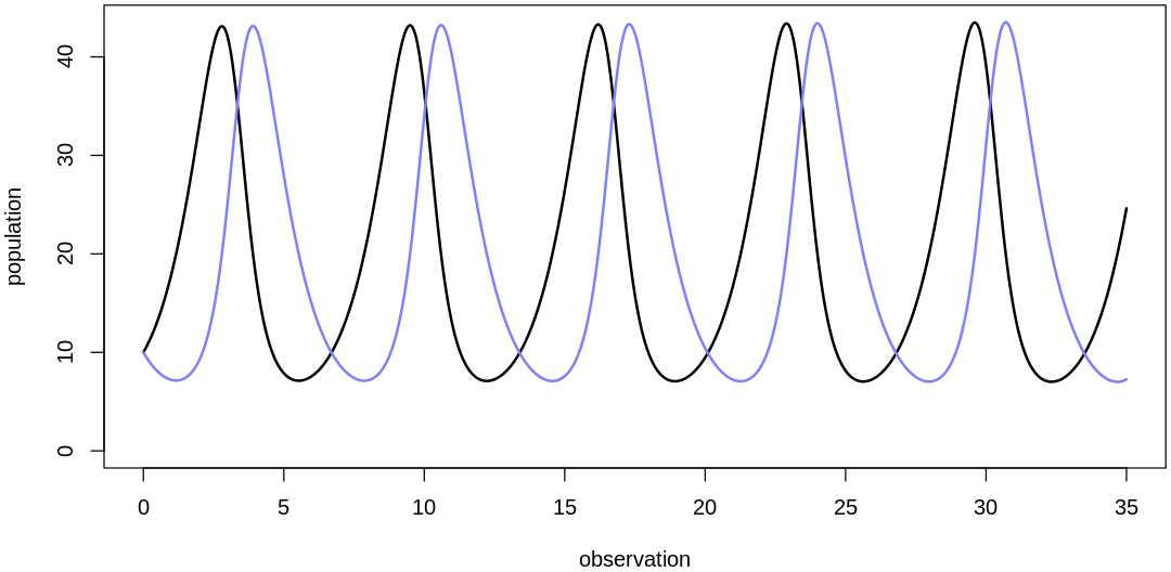
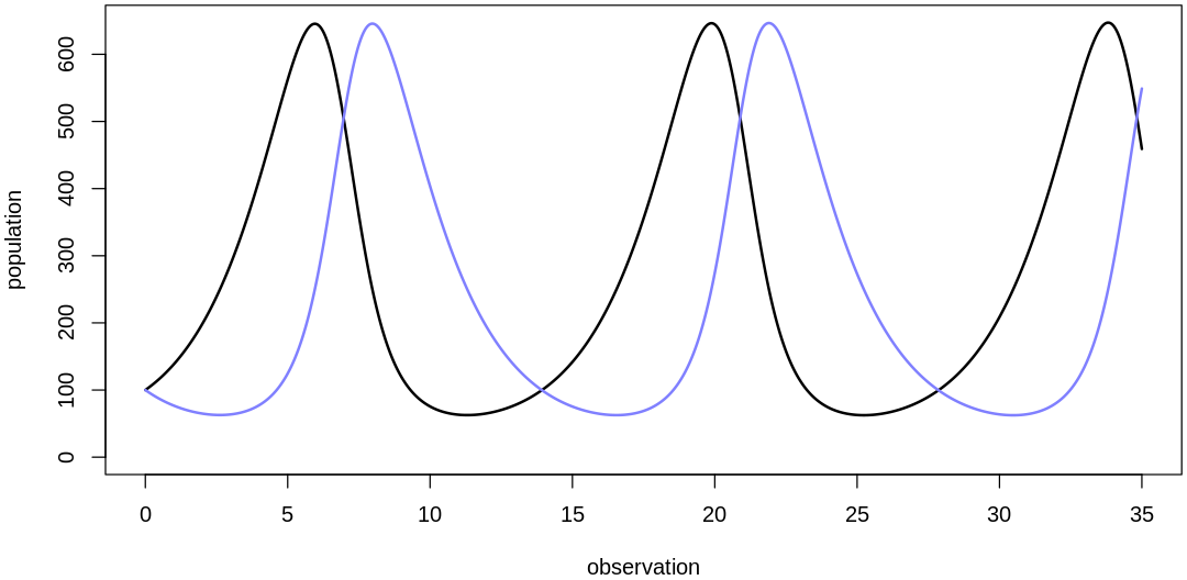
plot.mite.prior <- function(init, theta) {
  iplot(function() {
    par(mar = c(4.0, 4.0, 0.2, 0.2))
    n_sim <- 3.5e4
    dt <- 0.001
    z <- sim.pred.prey(n_sim, as.numeric(init), as.numeric(theta), dt=dt)
    t <- dt*(1:n_sim)
    display(init) 
    display(theta) 
    plot(t, z[, 2],
      type = "l", ylim = c(0, max(z[,])), lwd = 2,
      xlab="observation", ylab="population"
    )
    lines(t, z[, 1], col = rangi2, lwd = 2)
  }, ar=2)
}

Let’s select Mites priors starting from the Lynx-Hare model priors:

theta <- list(bPrey=1, mPrey=0.05, bPred=0.05, mPred=1)
init <- list(initPred=10, initPrey=10)
plot.mite.prior(init, theta)
init <- list(initPred=100, initPrey=100)
display_markdown("Scaling initial values:")
plot.mite.prior(init, theta)

$initPred

10

$initPrey

10

$bPrey

1

$mPrey

0.05

$bPred

0.05

$mPred

1

Scaling initial values:

$initPred

100

$initPrey

100

$bPrey

1

$mPrey

0.05

$bPred

0.05

$mPred

1

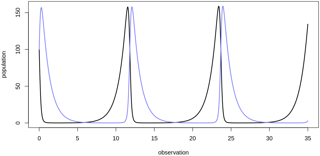
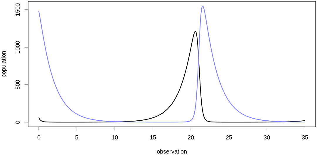
The two populations are starting to hit extreme values, unacceptable in a population model. To fix this, let’s reduce the two parameters associated with the coupling between the populations, \(m_{Prey}\) and \(b_{Pred}\). If we were to decrease these parameters to zero we would completely decouple the populations; we’ll pick something less extreme:

theta <- list(bPrey=1, mPrey=0.02, bPred=0.02, mPred=1)
plot.mite.prior(init, theta)

$initPred

100

$initPrey

100

$bPrey

1

$mPrey

0.02

$bPred

0.02

$mPred

1

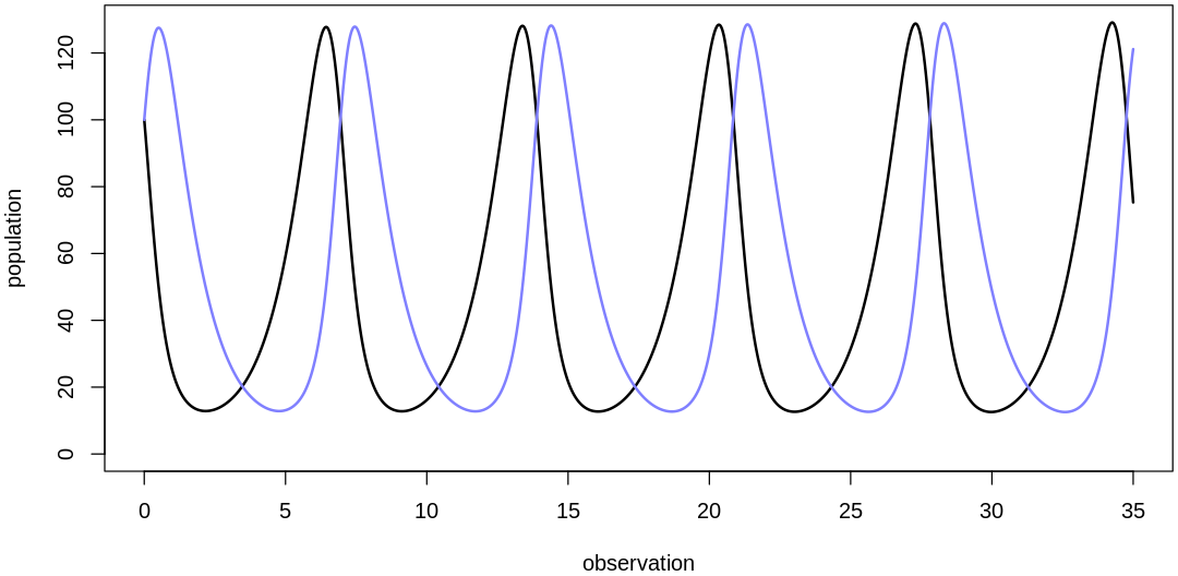
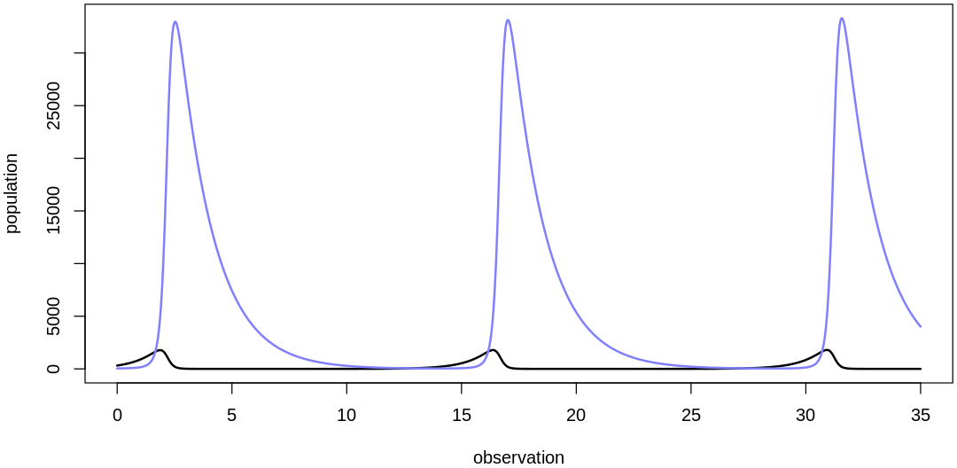
We’ve recovered more normal cycles, but the prediction scale is still low. Let’s increase birth rates to further increase the implied predictions:

theta <- list(bPrey=5, mPrey=0.02, bPred=0.02, mPred=5)
plot.mite.prior(init, theta)

$initPred

100

$initPrey

100

$bPrey

5

$mPrey

0.02

$bPred

0.02

$mPred

5

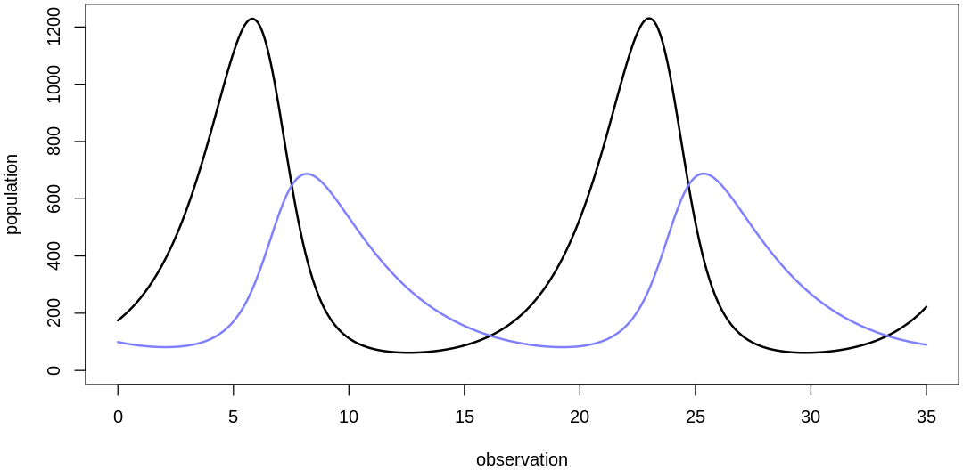
At this point we’re getting predictions on about the right output scale but this prior assumes mite populations change too quickly. If you look at the raw data you’ll see what looks like at most 5-6 cycles over the course of the 35 observations; if there were many more cycles we’d fail to capture them with data at this frequency anyways (see Nyquist rate).

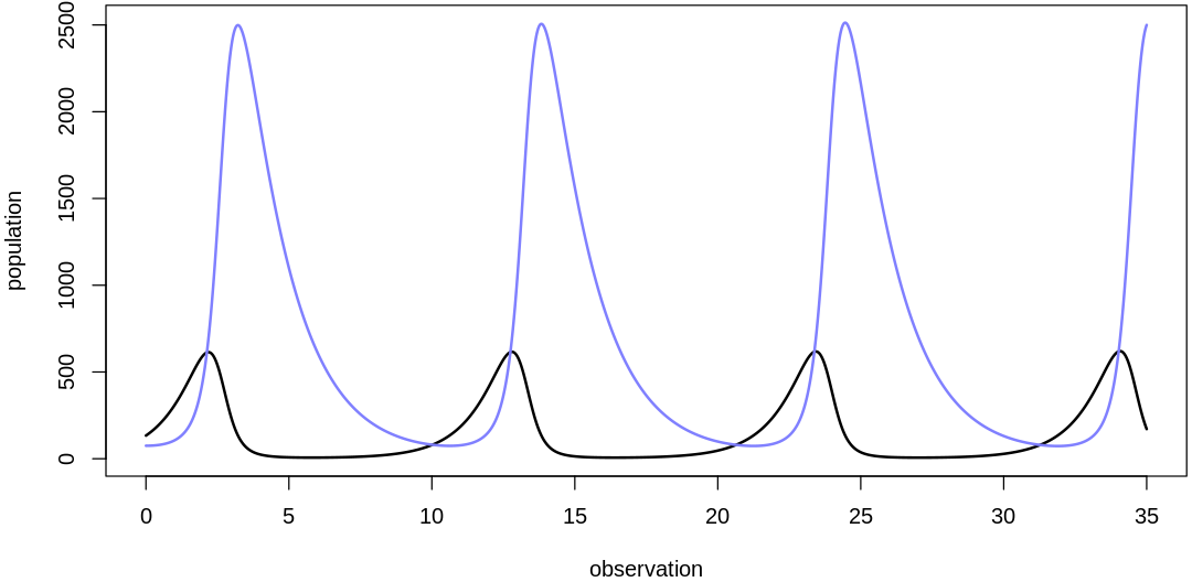
To decrease the rate at which the populations change, let’s inspect the original differential equations. Using the variable names on Lotka-Volterra equations, we want to decrease both \(dx/dt\) and \(dy/dt\). These rates are direct functions of all four parameters; to decrease them we can decrease our four main parameters:

theta <- list(bPrey=0.5, mPrey=0.002, bPred=0.002, mPred=0.5)
plot.mite.prior(init, theta)

$initPred

100

$initPrey

100

$bPrey

0.5

$mPrey

0.002

$bPred

0.002

$mPred

0.5

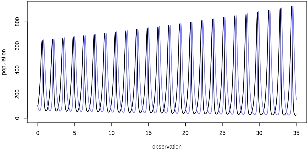
english.select.mites.prior.uncertainties <- r"(
<br/>
We've selected reasonable location parameters for our priors. Selecting the scale parameters is less
difficult; we'll skip those details and confirm that the combination of our scale and location
parameters (with a reasonable initial value prior) produces reasonable overall results. The next
five plots sample from the fully-specified prior:
)"

sim.mites.priors <- function() {
  display_markdown(english.select.mites.prior.uncertainties)
  set.seed(7)
  N <- 5
  iPred_sim <- rlnorm(N, meanlog=log(150), sdlog=1)
  iPrey_sim <- rlnorm(N, meanlog=log(150), sdlog=1)
  bPrey_sim <- abs(rnorm(N, mean=0.5, sd=0.2))
  mPrey_sim <- abs(rnorm(N, mean=0.002, sd=0.002))
  bPred_sim <- abs(rnorm(N, mean=0.002, sd=0.002))
  mPred_sim <- abs(rnorm(N, mean=0.5, sd=0.2))
  for (i in 1:length(bPrey_sim)) {
    init <- list(initPred=iPred_sim[i], initPrey=iPrey_sim[i])
    theta <- list(bPrey=bPrey_sim[i], mPrey=mPrey_sim[i], bPred=bPred_sim[i], mPred=mPred_sim[i])
    plot.mite.prior(init, theta)
  }
}
sim.mites.priors()

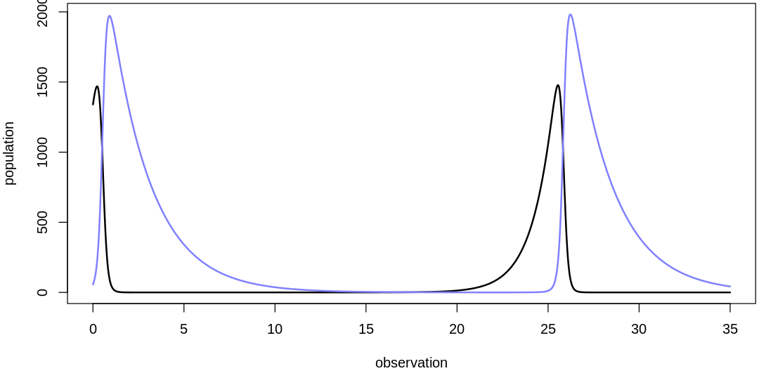
We've selected reasonable location parameters for our priors. Selecting the scale parameters is less difficult; we'll skip those details and confirm that the combination of our scale and location parameters (with a reasonable initial value prior) produces reasonable overall results. The next five plots sample from the fully-specified prior:

$initPred

1477.16864300832

$initPrey

58.1691618313371

$bPrey

0.571397246065805

$mPrey

0.0029353610226434

$bPred

0.00367950071924814

$mPred

0.536838554247153

$initPred

45.3252200639695

$initPrey

316.959699343477

$bPrey

1.04335035662614

$mPrey

0.000212398553829112

$bPred

0.003410683661811

$mPred

0.650455979148007

$initPred

74.9141494323312

$initPrey

133.44375366644

$bPrey

0.956290385197911

$mPrey

0.00138534340092561

$bPred

0.00461192944162338

$mPred

0.618349010492545

$initPred

99.3195413730304

$initPrey

174.738910588358

$bPrey

0.564804108027703

$mPrey

0.00199035515546486

$bPred

0.000775992433185701

$mPred

0.303389480845796

$initPred

56.824180773414

$initPrey

1340.25262517435

$bPrey

0.879213413361986

$mPrey

0.00397632829899989

$bPred

0.00454583372851047

$mPred

0.444787208977599

english.plot.mites.together <- r"(
<br/>
If we plot many posterior predictions (pairs of predator/prey traces) on a single plot as in the
text, it can be hard to identify which belong together:
)"
plot.combined.mites.posteriors <- function(d, prey_pred, pred_pred) {
  iplot(function() {
    N = length(d$day)
    plot(1:N, d$prey,
      main = "Combined Mites Posterior Predictions", pch = 16,
      ylim = c(0, max(d$prey)*1.05),
      xlab = "observation", ylab = "population"
    )
    points(1:N, d$predator, col = rangi2, pch = 16)
    for (s in 1:20) {
      lines(1:N, prey_pred[s,], col = col.alpha("black", 0.2), lwd = 2)
      lines(1:N, pred_pred[s,], col = col.alpha(rangi2, 0.3), lwd = 2)
    }
  })
}
english.plot.mites.separate <- r"(
<br/>
Let's take five snapshots of individual pairs instead:
)"
plot.separate.mites.posteriors <- function(d, prey_pred, pred_pred) {
  N = length(d$day)
  for (s in 1:5) {
    iplot(function() {
      plot(1:N, d$prey,
        main = paste("Mites Posterior Predictions #", s, sep=""), pch = 16,
        ylim = c(0, max(d$prey)*1.05),
        xlab = "observation", ylab = "population"
      )
      points(1:N, d$predator, col = rangi2, pch = 16)
      lines(1:N, prey_pred[s,], col = col.alpha("black", 0.2), lwd = 2)
      lines(1:N, pred_pred[s,], col = col.alpha(rangi2, 0.3), lwd = 2)
    })
  }
}
fit.mites.model <- function(d) {
  dat_list <- list(
    N = nrow(d),
    pelts = d[, 3:2]
  )
  m.mites <- stan(
    file = "mites.stan", data = dat_list,
    chains = 4, cores = 4, seed = 14,
    control = list(adapt_delta = 0.95)
  )
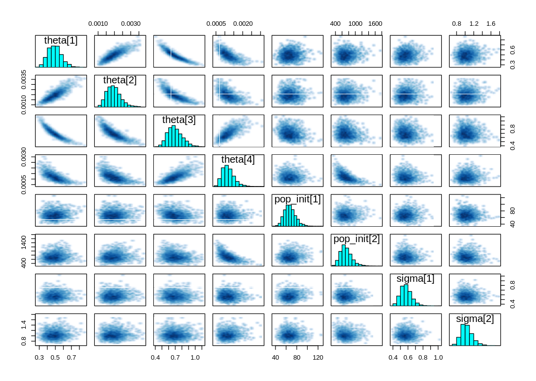
  display_markdown("A `pairs` plot: ")
  iplot(function() {
    pairs(m.mites, pars=c("theta", "pop_init", "sigma"))
  })
  flush.console()
  post <- extract.samples(m.mites)
  prey_pred = post$pop_pred[,,2]
  pred_pred = post$pop_pred[,,1]
  display_markdown(english.plot.mites.together)
  plot.combined.mites.posteriors(d, prey_pred, pred_pred)
  display_markdown(english.plot.mites.separate)
  plot.separate.mites.posteriors(d, prey_pred, pred_pred)
}
fit.mites.model(d)

A pairs plot:

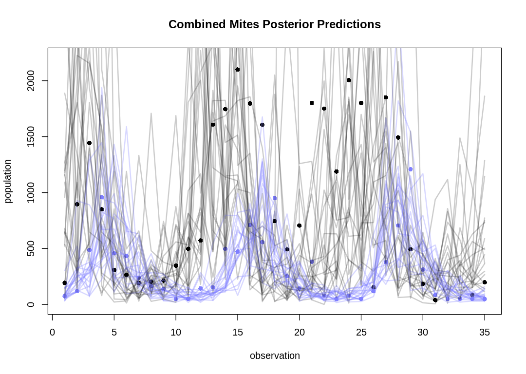
If we plot many posterior predictions (pairs of predator/prey traces) on a single plot as in the text, it can be hard to identify which belong together:
Let's take five snapshots of individual pairs instead:

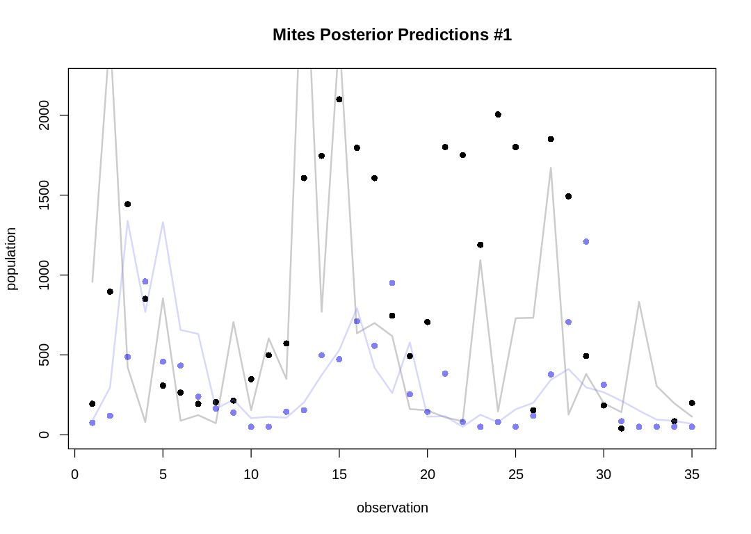
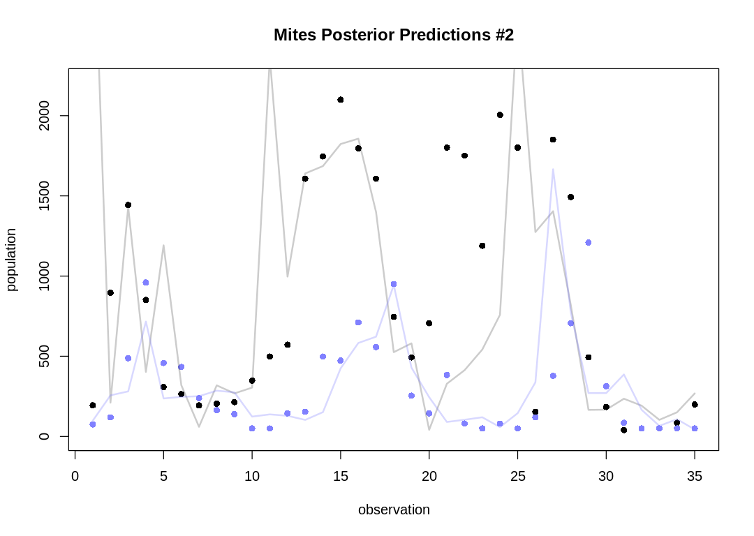
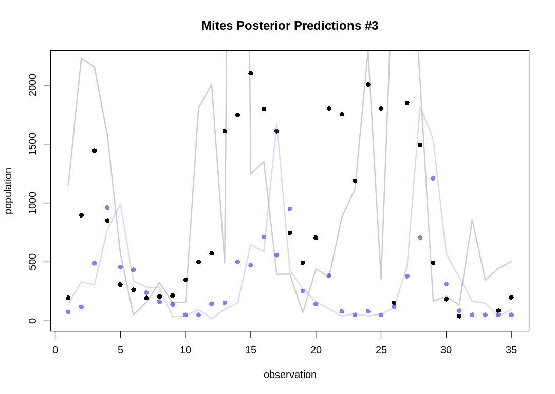
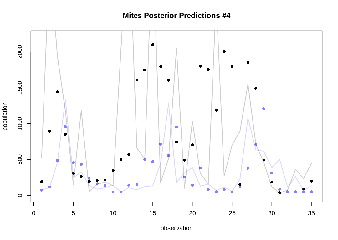
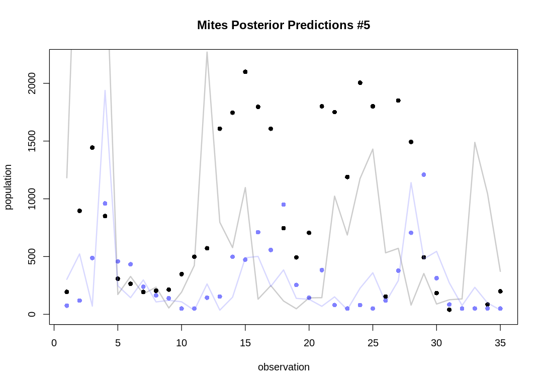
As expected, the Lotka-Volterra model doesn’t fit nearly as well to this data as it did to the Lynx-Hare data.