2.3. Enrichment#
from IPython.display import Image
2.3.1. 𝓥-categories#

Define enriched preorder#
A 𝓥-category is a generalization of a category, see Enriched category. However, the definition given in this section is not of an enriched category (as Wikipedia gives it); see section 4.4.4. for that definition.
In the context of Chp. 2 we can define “the” hom-object (in the language of Definition 2.46, defining a 𝓥-category) as a boolean or real number. In a Set-category (a regular category) we could say “the” hom-object is a set and hence we call it a hom-set. When we say “the” hom-element (in the language of Definition 2.79, defining a closed monoidal preorder) we are talking about \(v ⊸ w\), which is only the same as the hom-object if the category is self-enriched (see Remark 2.89).
With either understanding you can see enrichment as labeling the edges of a graph; the hom-object is the label. However, this labelling has to be done in a way that respects e.g. the triangle equality.
You should usually read 𝓥-category as “monoidal category” rather than “V category” audibly, only because it is more semantically meaningful. The author actually defines it to mean “symmetric monoidal category” in Chp. 2; and in addition only deals with the special case of preorders.
To remember part (b) of this definition at this point, you should really think of it in terms of Bool: if x ≤ y and y ≤ x, then x ≤ z. In Chp. 4 we’ll see how it effectively defines composition.
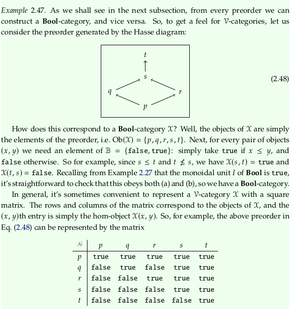
2.3.2. Preorders as Bool-categories#
See also Examples of enriched categories.
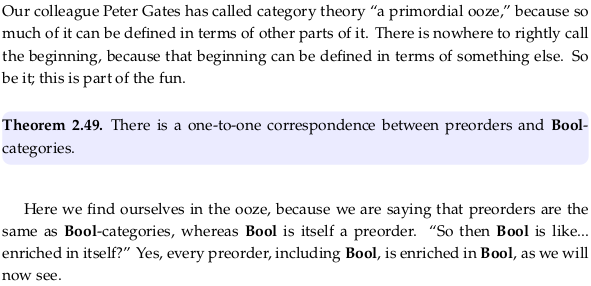
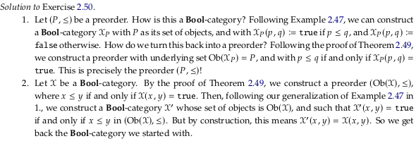
Exercise 2.50.#
See also Exercise 2.50.
Image('raster/2023-10-28T18-30-18.png', metadata={'description': "7S answer"})

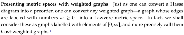
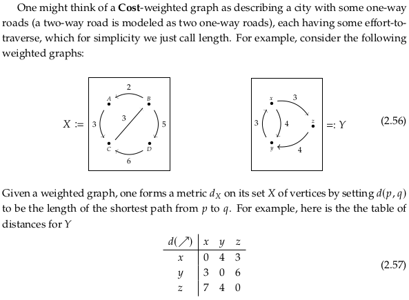
2.3.3. Lawvere metric spaces#

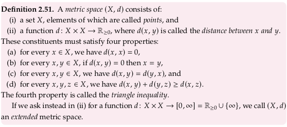
See also Pseudoquasimetrics. Dropping (b) in Definition 2.51 is equivalent to adding the “pseudo” prefix and dropping (c) is equivalent to adding the “quasi” prefix.
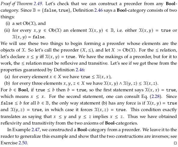
Exercise 2.52.#

Image('raster/2023-10-28T18-30-49.png', metadata={'description': "7S answer"})

Define Hausdorff distance#
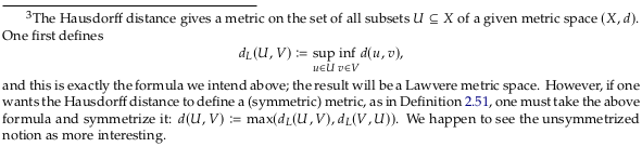
See also Hausdorff distance. If you’re not familiar with inf being used in an equation, this may be hard to swallow. Let’s start with the simpler definition of Closeness (mathematics). The distance between a point and a set is defined as:
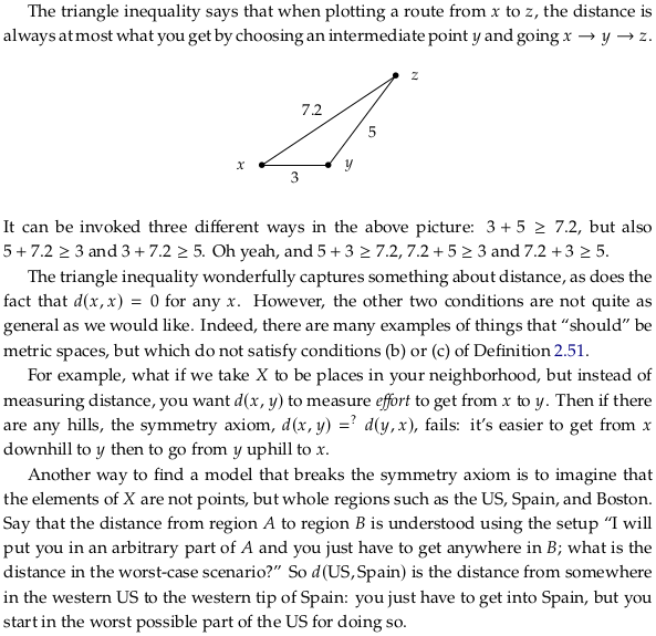
A picture to have in mind (with a few example distances) is:

We take the infimum of the blue line (which is about 3) to get the distance between the point and the set.
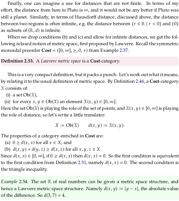
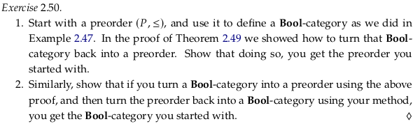
Exercise 2.55.#
Image('raster/2023-10-28T18-31-23.png', metadata={'description': "7S answer"})

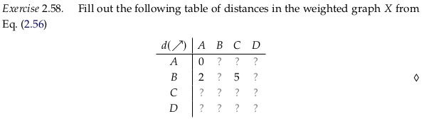
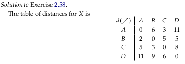
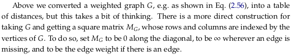
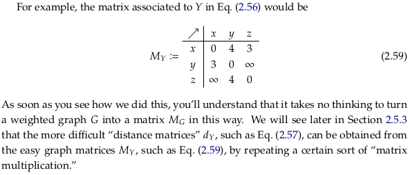
Exercise 2.58.#
Image('raster/2023-10-28T18-31-54.png', metadata={'description': "7S answer"})
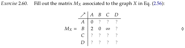
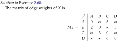
Exercise 2.60.#
Image('raster/2023-10-28T18-32-12.png', metadata={'description': "7S answer"})
2.3.4. 𝓥-variations on preorders and metric spaces#
import pandas as pd

def prove_v_category(df, mon_prod, preorder_rel):
    for row in df.index:
        for col in df.columns:
            for idx in range(0,len(df.index)):
                a = mon_prod(df.iloc[row, idx], df.iloc[idx, col])
                assert preorder_rel(a, df.iloc[row,col]), (row,idx,col)
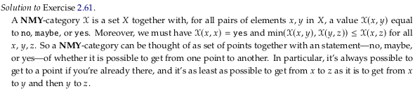
Exercise 2.61.#

See also Exercise 2.61.
Image('raster/2023-10-27T17-26-22.png', metadata={'description': "7S answer"})

Exercise 2.62.#
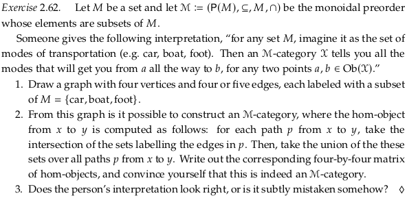
See also Exercise 2.62.
Image('raster/2023-10-27T17-30-23.png', metadata={'description': "7S answer"})
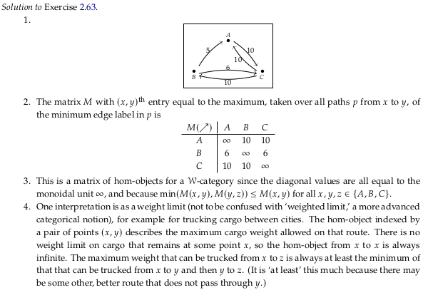
Exercise 2.63.#
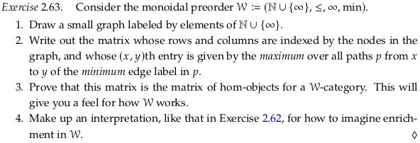
See also Exercise 2.63.
Image('raster/2023-10-29T21-41-19.png', metadata={'description': "7S answer"})