Practice: Chp. 12

source("iplot.R")
suppressPackageStartupMessages(library(rethinking))

12E1. What is the difference between an ordered categorical variable and an unordered one? Define and then give an example of each.

Answer. An ordered categorical variable is one in which the categories are ranked, but the distance between the categories is not necessarily constant. An example of an ordered categorical variable is the Likert scale; an example of an unordered categorical variable is the Blood type of a person.

See also Categorical variable and Ordinal data.

12E2. What kind of link function does an ordered logistic regression employ? How does it differ from an ordinary logit link?

Answer. It employs a cumulative link, which maps the probability of a category or any category of lower rank (the cumulative probability) to the log-cumulative-odds scale. The major difference from the ordinary logit link is the type of probabilties being mapped; the cumulative link maps cumulative probabilities to log-cumulative-odds and the ordinary logit link maps absolute probabilities to log-odds.

12E3. When count data are zero-inflated, using a model that ignores zero-inflation will tend to induce which kind of inferential error?

Answer. A ‘zero’ means that nothing happened; nothing can happen either because the rate of events is low because the process that generates events failed to get started. We may incorrectly infer the rate of events is lower than it is in reality, when in fact it never got started.

12E4. Over-dispersion is common in count data. Give an example of a natural process that might produce over-dispersed counts. Can you also give an example of a process that might produce under-dispersed counts?

Answer. The sex ratios of families actually skew toward either all boys or girls; see Overdispersion.

In contexts where the waiting time for a service is bounded (e.g. a store is only open a short time) but the model still uses a Poisson distribution you may see underdispersed counts because large values are simply not possible. If one queue feeds into another, and the first queue has a limited number of workers, the waiting times for the second queue may be underdispersed because of the homogeneity enforced by the bottleneck in the first queue. “)

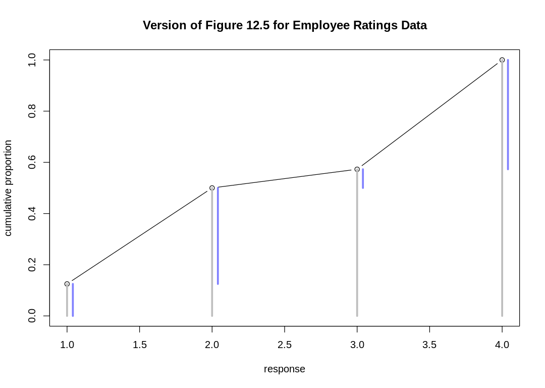
display_markdown(” 12M1. At a certain university, employees are annually rated from 1 to 4 on their productivity, with 1 being least productive and 4 most productive. In a certain department at this certain university in a certain year, the numbers of employees receiving each rating were (from 1 to 4): 12, 36, 7, 41. Compute the log cumulative odds of each rating.

Answer. As a list:

freq_prod <- c(12, 36, 7, 41)
pr_k <- freq_prod / sum(freq_prod)
cum_pr_k <- cumsum(pr_k)
lco = list(log_cum_odds = logit(cum_pr_k))
display(lco)

$log_cum_odds =

1. -1.94591014905531
2. 0
3. 0.293761118528163
4. Inf

12M2. Make a version of Figure 12.5 for the employee ratings data given just above.

iplot(function() {
  off <- 0.04
  plot(
    1:4, cum_pr_k, type="b",
    main="Version of Figure 12.5 for Employee Ratings Data", xlab="response", ylab="cumulative proportion",
    ylim=c(0,1)
  )
  # See `simplehist`
  for (j in 1:4) lines(c(j,j), c(0,cum_pr_k[j]), lwd=3, col="gray")
  for (j in 1:4) lines(c(j,j)+off, c(if (j==1) 0 else cum_pr_k[j-1],cum_pr_k[j]), lwd=3, col=rangi2)
})

12M3. Can you modify the derivation of the zero-inflated Poisson distribution (ZIPoisson) from the chapter to construct a zero-inflated binomial distribution?

Answer. Call \(p_z\) the additional probability of a zero, and \(p_b\) the probability of success associated with the binomial distribution. The likelihood of observing a zero is:

\[\begin{split} \begin{align} Pr(0 | p_z,n,p_b) & = p_z + (1-p_z)Pr(0|n,p_b) \\ & = p_z + (1-p_z)\binom{n}{0}p_b^0(1-p_b)^{n-0} \\ & = p_z + (1-p_z)(1-p_b)^n \end{align} \end{split}\]

The likelihood of observing a non-zero value \(k\) is: $\( \begin{align} Pr(k | k>0,p_z,n,p_b) & = (1-p_z)Pr(k|n,p_b) \\ & = (1-p_z)\binom{n}{k}p_b^k(1-p_b)^{n-k} \end{align} \)$

To construct a GLM, use a logit link with \(p_z\) and \(p_b\) (in the typical case where \(n\) is known).

12H1. In 2014, a paper was published that was entitled “Female hurricanes are deadlier than male hurricanes.” As the title suggests, the paper claimed that hurricanes with female names have caused greater loss of life, and the explanation given is that people unconsciously rate female hurricanes as less dangerous and so are less likely to evacuate.

Statisticians severely criticized the paper after publication. Here, you’ll explore the complete data used in the paper and consider the hypothesis that hurricanes with female names are deadlier. Load the data with:

R code 12.38

library(rethinking)
data(Hurricanes)

Acquaint yourself with the columns by inspecting the help ?Hurricanes. In this problem, you’ll focus on predicting deaths using femininity of each hurricane’s name. Fit and interpret the simplest possible model, a Poisson model of deaths using femininity as a predictor. You can use map or ulam. Compare the model to an intercept-only Poisson model of deaths. How strong is the association between femininity of name and deaths? Which storms does the model fit (retrodict) well? Which storms does it fit poorly?

Answer. The Hurricanes data.frame with an index and a standardized femininity:

data(Hurricanes)
hur <- Hurricanes
hur$index = 1:92
hur$StdFem = standardize(hur$femininity)
display(hur)

hur_dat = list(
  Deaths = hur$deaths,
  Femininity = hur$StdFem
)

m_hur_pois <- map(
  alist(
    Deaths ~ dpois(lambda),
    log(lambda) <- a + bFemininity * Femininity,
    a ~ dnorm(3, 0.5),
    bFemininity ~ dnorm(0, 1.0)
  ),
  data = hur_dat
)

m_hur_intercept <- map(
  alist(
    Deaths ~ dpois(lambda),
    log(lambda) <- a,
    a ~ dnorm(3, 0.5)
  ),
  data = hur_dat
)

A data.frame: 92 × 10

name	year	deaths	category	min_pressure	damage_norm	female	femininity	index	StdFem
<fct>	<int>	<int>	<int>	<int>	<int>	<int>	<dbl>	<int>	<dbl>
Easy	1950	2	3	960	1590	1	6.77778	1	-0.0009347453
King	1950	4	3	955	5350	0	1.38889	2	-1.6707580424
Able	1952	3	1	985	150	0	3.83333	3	-0.9133139565
Barbara	1953	1	1	987	58	1	9.83333	4	0.9458703621
Florence	1953	0	1	985	15	1	8.33333	5	0.4810742824
Carol	1954	60	3	960	19321	1	8.11111	6	0.4122162926
Edna	1954	20	3	954	3230	1	8.55556	7	0.5499353710
Hazel	1954	20	4	938	24260	1	9.44444	8	0.8253673305
Connie	1955	0	3	962	2030	1	8.50000	9	0.5327193242
Diane	1955	200	1	987	14730	1	9.88889	10	0.9630864089
Ione	1955	7	3	960	6200	0	5.94444	11	-0.2591568553
Flossy	1956	15	2	975	1540	1	7.00000	12	0.0679232445
Helene	1958	1	3	946	540	1	9.88889	13	0.9630864089
Debra	1959	0	1	984	430	1	9.88889	14	0.9630864089
Gracie	1959	22	3	950	510	1	9.77778	15	0.9286574139
Donna	1960	50	4	930	53270	1	9.27778	16	0.7737253874
Ethel	1960	0	1	981	35	1	8.72222	17	0.6015773141
Carla	1961	46	4	931	15850	1	9.50000	18	0.8425833773
Cindy	1963	3	1	996	300	1	9.94444	19	0.9802993570
Cleo	1964	3	2	968	6450	1	7.94444	20	0.3605712508
Dora	1964	5	2	966	16260	1	9.33333	21	0.7909383355
Hilda	1964	37	3	950	2770	1	8.83333	22	0.6360063090
Isbell	1964	3	2	974	800	1	9.44444	23	0.8253673305
Betsy	1965	75	3	948	20000	1	8.33333	24	0.4810742824
Alma	1966	6	2	982	730	1	8.77778	25	0.6187933608
Inez	1966	3	1	983	99	1	8.27778	26	0.4638613343
Beulah	1967	15	3	950	5060	1	7.27778	27	0.1539972812
Gladys	1968	3	2	977	800	1	8.94444	28	0.6704353039
Camille	1969	256	5	909	23040	1	9.05556	29	0.7048673975
Celia	1970	22	3	945	6870	1	9.44444	30	0.8253673305
⋮	⋮	⋮	⋮	⋮	⋮	⋮	⋮	⋮	⋮
Bertha	1996	8	2	974	700	1	8.50000	63	0.5327193
Fran	1996	26	3	954	8260	1	7.16667	64	0.1195683
Danny	1997	10	1	984	200	0	2.22222	65	-1.4125390
Bonnie	1998	3	2	964	1650	1	9.38889	66	0.8081544
Earl	1998	3	1	987	160	0	1.88889	67	-1.5158260
Georges	1998	1	2	964	3870	0	2.27778	68	-1.3953230
Bret	1999	0	3	951	94	0	2.33333	69	-1.3781100
Floyd	1999	56	2	956	8130	0	1.83333	70	-1.5330421
Irene	1999	8	1	964	1430	1	9.27778	71	0.7737254
Lili	2002	2	1	963	1260	1	10.33333	72	1.1008024
Claudette	2003	3	1	979	250	1	9.16667	73	0.7392964
Isabel	2003	51	2	957	4980	1	9.38889	74	0.8081544
Alex	2004	1	1	972	5	0	4.16667	75	-0.8100239
Charley	2004	10	4	941	20510	0	2.88889	76	-1.2059620
Frances	2004	7	2	960	12620	1	6.00000	77	-0.2419408
Gaston	2004	8	1	985	170	0	2.66667	78	-1.2748200
Ivan	2004	25	3	946	18590	0	1.05556	79	-1.7740450
Jeanne	2004	5	3	950	10210	1	8.50000	80	0.5327193
Cindy	2005	1	1	991	350	1	9.94444	81	0.9802994
Dennis	2005	15	3	946	2650	0	2.44444	82	-1.3436810
Ophelia	2005	1	1	982	91	1	9.16667	83	0.7392964
Rita	2005	62	3	937	10690	1	9.50000	84	0.8425834
Wilma	2005	5	3	950	25960	1	8.61111	85	0.5671483
Humberto	2007	1	1	985	51	0	2.38889	86	-1.3608940
Dolly	2008	1	1	967	1110	1	9.83333	87	0.9458704
Gustav	2008	52	2	954	4360	0	1.72222	88	-1.5674711
Ike	2008	84	2	950	20370	0	1.88889	89	-1.5158260
Irene	2011	41	1	952	7110	1	9.27778	90	0.7737254
Isaac	2012	5	1	966	24000	0	1.94444	91	-1.4986131
Sandy	2012	159	2	942	75000	1	9.00000	92	0.6876514

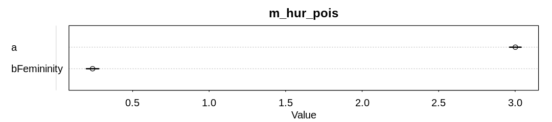
The model with the femininity predictor appears to have inferred a minor but significant association of deaths with femininity:

iplot(function() {
  plot(precis(m_hur_pois), main="m_hur_pois")
}, ar=4.5)

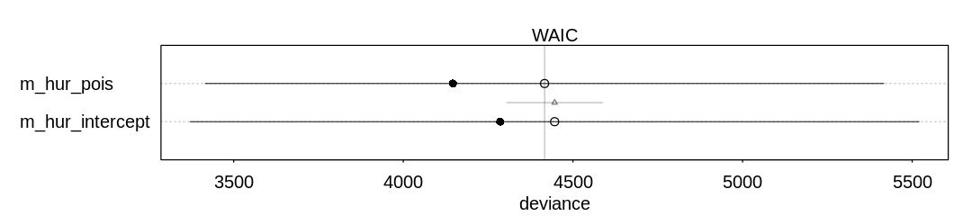
The model with the femininity predictor performs only marginally better on WAIC than the intercept-only model:

iplot(function() {
  plot(compare(m_hur_pois, m_hur_intercept))
}, ar=4.5)

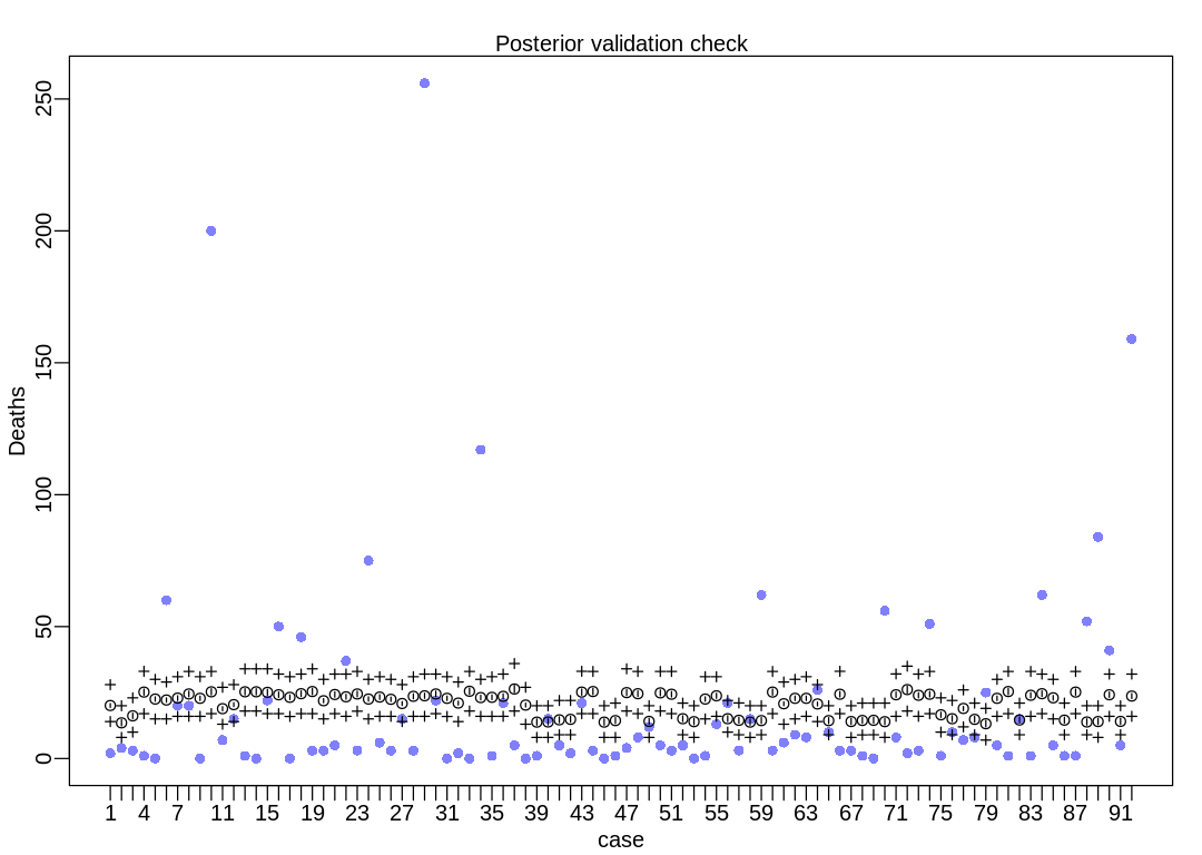
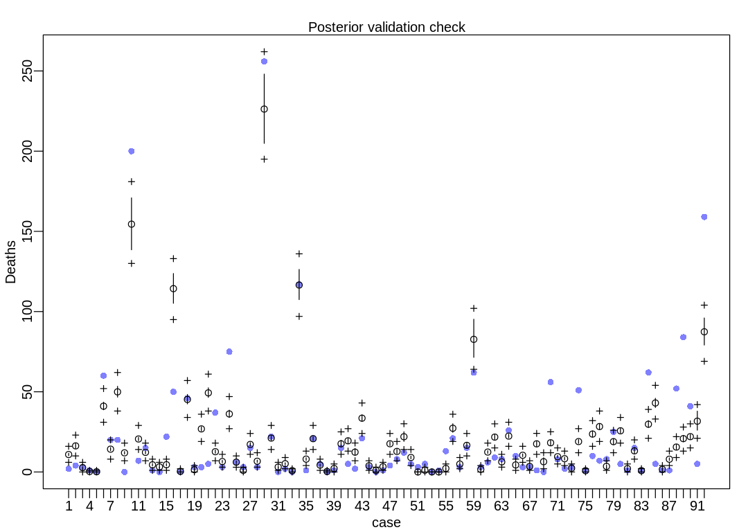
The model is not accurate when it attempts to retrodict the death toll on storms with many deaths. The predictions it makes are less dispersed than the data, that is, the data are overdispersed relative to the predictions (Overdispersion).

iplot(function() {
  result <- postcheck(m_hur_pois, window=92)
  display_markdown("The raw data:")
  display(result)
})

The raw data:

$mean

1. 20.0909638320166
2. 13.5143028318176
3. 16.1733109878181
4. 25.1787772660708
5. 22.5358282653805
6. 22.1689133858378
7. 22.908911670051
8. 24.464810148839
9. 22.8150541596038
10. 25.2824892298876
11. 18.8935278512169
12. 20.4230650001127
13. 25.2824892298876
14. 25.2824892298876
15. 25.0755146831786
16. 24.1651462880186
17. 23.1928029015675
18. 24.5655442972114
19. 25.3866150597648
20. 21.8976943074182
21. 24.2646129731868
22. 23.3840464063741
23. 24.464810148839
24. 22.5358282653805
25. 23.2882344448313
26. 22.4435351630679
27. 20.8460304273314
28. 23.5768871486183
29. 23.7713562060926
30. 24.464810148839
31. 22.8150541596038
32. 21.0176877923093
33. 25.4911940714126
34. 23.0977844592675
35. 23.1928029015675
36. 23.5768871486183
37. 26.3436111294371
38. 20.256325111861
39. 13.7926856723714
40. 13.8490494913378
41. 14.6631794659105
42. 14.8438538180013
43. 25.1787772660708
44. 25.3866150597648
45. 13.7926856723714
46. 14.366994702575
47. 24.972662491807
48. 24.5655442972114
49. 14.0768685409229
50. 24.8702559127626
51. 24.3645123304141
52. 15.0882588251682
53. 13.9624883489791
54. 22.5358282653805
55. 23.7713562060926
56. 15.0882588251682
57. 14.4847323337607
58. 13.7926856723714
59. 14.366994702575
60. 25.1787772660708
61. 20.7607272428806
62. 22.8150541596038
63. 22.8150541596038
64. 20.6757928318801
65. 14.366994702575
66. 24.3645123304141
67. 14.0195654325719
68. 14.425747144927
69. 14.4847323337607
70. 13.9624883489791
71. 24.1651462880186
72. 26.1278374211388
73. 23.9674321978027
74. 24.3645123304141
75. 16.5748764082044
76. 15.0882588251682
77. 18.9710650264949
78. 14.8438538180013
79. 13.1877497964257
80. 22.8150541596038
81. 25.3866150597648
82. 14.6034474230733
83. 23.9674321978027
84. 24.5655442972114
85. 23.0031432446451
86. 14.5439725264936
87. 25.1787772660708
88. 13.8490494913378
89. 14.0195654325719
90. 24.1651462880186
91. 14.0768685409229
92. 23.6739194496856

$PI

A matrix: 2 × 92 of type dbl

5%	19.36255	12.35423	15.17837	24.04287	21.72629	21.38360	22.05466	23.41482	21.96716	24.12438	⋯	23.00362	23.51569	22.14179	13.44805	24.04287	12.71166	12.88551	23.18141	12.94499	22.72557
94%	20.82471	14.72758	17.18187	26.33569	23.37489	22.96874	23.77376	25.52207	23.66849	26.46576	⋯	24.93669	25.63526	23.88443	15.68156	26.33569	15.04457	15.19707	25.16973	15.24818	24.61595

$outPI

A matrix: 2 × 92 of type dbl

5%	14	8	10	17.000	15	15	16	16	16	17	⋯	16	17	15	9	17	9	8	16	9	16
94%	28	20	23	33.055	30	29	31	33	31	33	⋯	33	32	30	21	33	20	20	32	20	32

12H2. Counts are nearly always over-dispersed relative to Poisson. So fit a gamma-Poisson (aka negative-binomial) model to predict deaths using femininity. Show that the over-dispersed model no longer shows as precise a positive association between femininity and deaths, with an 89% interval that overlaps zero. Can you explain why the association diminished in strength?

data(Hurricanes)
hur <- Hurricanes
hur$index = 1:92
hur$StdFem = standardize(hur$femininity)

hur_dat = list(
  Deaths = hur$deaths,
  Femininity = hur$StdFem
)

m_hur_gamma_pois <- map(
  alist(
    Deaths ~ dgampois(lambda, phi),
    log(lambda) <- a + bFemininity * Femininity,
    a ~ dnorm(3, 0.5),
    bFemininity ~ dnorm(0, 1.0),
    phi ~ dexp(1)
  ),
  data = hur_dat
)

Answer. The model no longer infers an association of deaths with femininity:

iplot(function() {
  plot(precis(m_hur_gamma_pois), main="m_hur_gamma_pois")
}, ar=4.5)

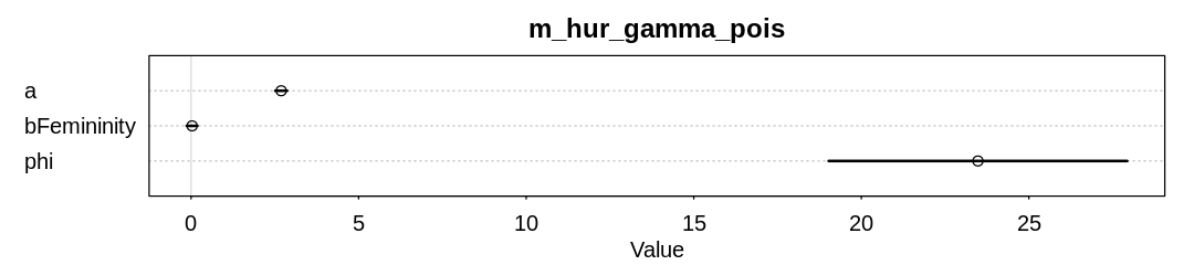
The association has diminished in strength because the influence of outliers are diminished. Notice the storms with the greatest death toll are female in the original data: Diane, Camille, and Sandy.

12H3. In the data, there are two measures of a hurricane’s potential to cause death: damage_norm and min_pressure. Consult ?Hurricanes for their meanings. It makes some sense to imagine that femininity of a name matters more when the hurricane is itself deadly. This implies an interaction between femininity and either or both of damage_norm and min_pressure. Fit a series of models evaluating these interactions. Interpret and compare the models. In interpreting the estimates, it may help to generate counterfactual predictions contrasting hurricanes with masculine and feminine names. Are the effect sizes plausible?

data(Hurricanes)
hur <- Hurricanes
hur$index = 1:92
hur$StdFem = standardize(hur$femininity)
hur$StdDam = standardize(hur$damage_norm)
hur$StdPres = standardize(hur$min_pressure)

Answer. To get some unreasonable answers, lets go back to the Poisson distribution rather than the Gamma-Poisson. It’s likely this is what the authors of the original paper were using.

hur_dat = list(
  Deaths = hur$deaths,
  StdFem = hur$StdFem,
  StdDam = hur$StdDam
)

m_fem_dam_inter <- quap(
  alist(
    Deaths ~ dpois(lambda),
    log(lambda) <- a + bFem * StdFem + bDam * StdDam + bFemDamInter * StdFem * StdDam,
    a ~ dnorm(3, 0.5),
    bFem ~ dnorm(0, 1.0),
    bDam ~ dnorm(0, 1.0),
    bFemDamInter ~ dnorm(0, 0.4)
  ),
  data = hur_dat
)

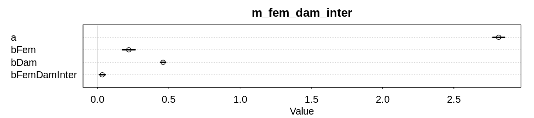
In the first model, lets assume an interaction between femininity and damage_norm. Damage is unsurprisingly associated with more deaths. The model also believes there is a minor interaction between damage and femininity, where together they increase deaths more than either alone.

iplot(function() {
  plot(precis(m_fem_dam_inter), main="m_fem_dam_inter")
}, ar=4.5)

hur_dat = list(
  Deaths = hur$deaths,
  StdFem = hur$StdFem,
  StdPres = hur$StdPres
)

m_fem_pres_inter <- quap(
  alist(
    Deaths ~ dpois(lambda),
    log(lambda) <- a + bFem * StdFem + bPres * StdPres + bFemPresInter * StdFem * StdPres,
    a ~ dnorm(3, 0.5),
    bFem ~ dnorm(0, 1.0),
    bPres ~ dnorm(0, 1.0),
    bFemPresInter ~ dnorm(0, 0.4)
  ),
  data = hur_dat
)

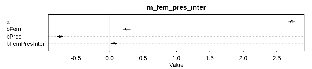
In the second model, lets assume an interaction between femininity and min_pressure. Pressure is unsurprisingly negatively associated with more deaths; lower pressure indicates a stronger storm. There also appears to be a minor interaction between pressure and femininity, though now the association is in the opposite direction. That is, when both pressure and femininity are positive, which means the storm is weak and feminine, more deaths occur.

iplot(function() {
  plot(precis(m_fem_pres_inter), main="m_fem_pres_inter")
}, ar=4.5)

hur_dat = list(
  Deaths = hur$deaths,
  StdFem = hur$StdFem,
  StdPres = hur$StdPres,
  StdDam = hur$StdDam
)

m_fem_dam_pres_inter <- quap(
  alist(
    Deaths ~ dpois(lambda),
    log(lambda) <- a + bFem * StdFem + bPres * StdPres + bDam * StdDam +
        bFemPresInter * StdFem * StdPres +
        bFemDamInter * StdFem * StdDam +
        bDamPresInter * StdDam * StdPres +
        bFDPInter * StdPres * StdDam * StdPres,
    a ~ dnorm(3, 0.5),
    bFem ~ dnorm(0, 1.0),
    bDam ~ dnorm(0, 1.0),
    bPres ~ dnorm(0, 1.0),
    bFemPresInter ~ dnorm(0, 0.4),
    bFemDamInter ~ dnorm(0, 0.4),
    bDamPresInter ~ dnorm(0, 0.4),
    bFDPInter ~ dnorm(0, 0.4)
  ),
  data = hur_dat
)

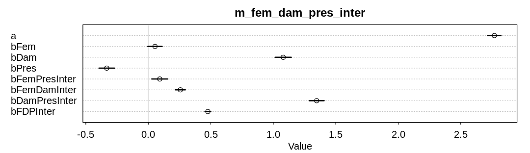
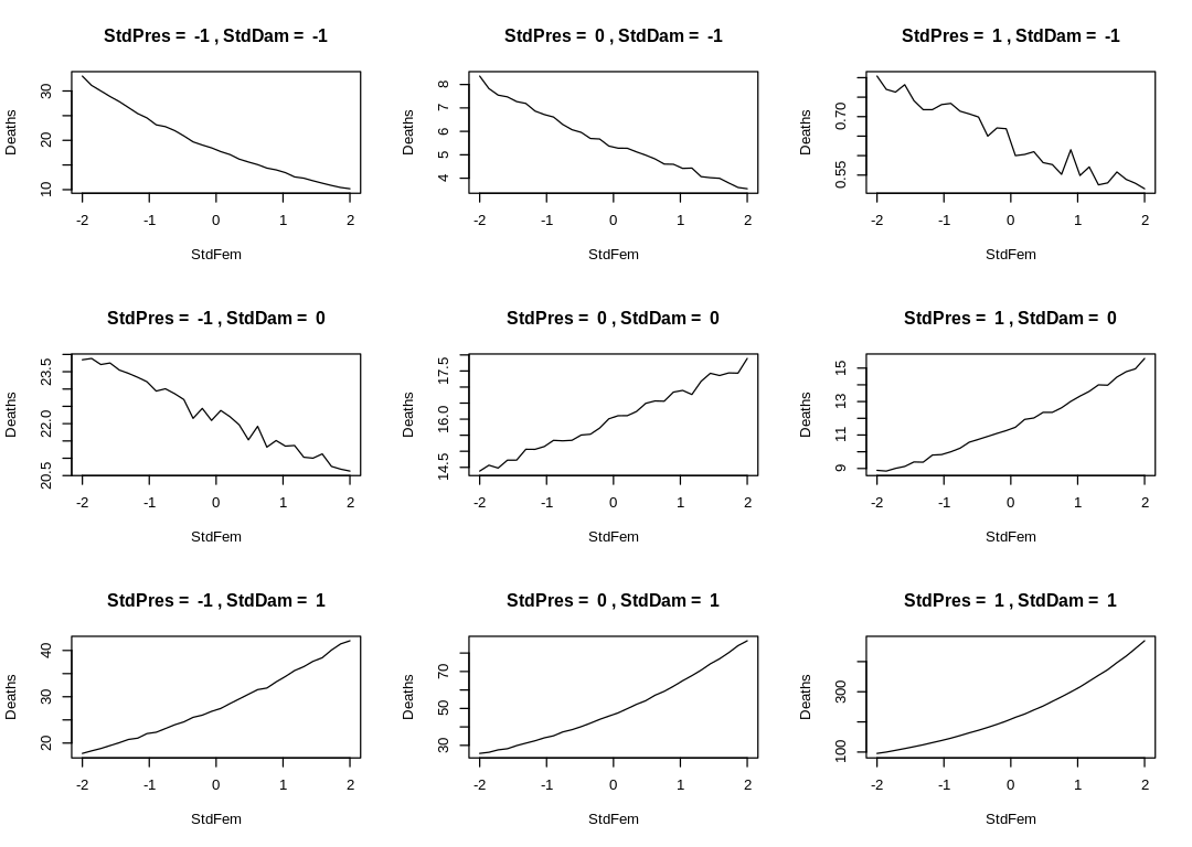
In the third model, lets assume interactions between all three predictors. The influence of femininity has dropped significantly. The three-way interaction term is hard to interpret on the parameter scale. Lets try to interpret it on the outcome scale.

iplot(function() {
  plot(precis(m_fem_dam_pres_inter), main="m_fem_dam_pres_inter")
}, ar=3.5)

To some extent this is a counterfactual plot rather than just a posterior prediction plot because we’re considering extremes of at least some predictors. Still, many of the predictors vary here only within the range of the data.

In the following Enneaptych, we hold damage and pressure at typical values and vary femininity. We observe the effect on deaths. Many of the effect sizes are inplausible. In the bottom-right plot, notice an implication of the non-negative three-way interaction parameter: when pressure is high and damage is low femininity has a dramatic effect on deaths.

iplot(function() {
  par(mfrow=c(3,3))
  for (d in -1: 1) {
    for (p in -1:1) {
      sim_dat = data.frame(StdPres=p, StdDam=d, StdFem=seq(from=-2, to=2, length.out=30))
      s <- sim(m_fem_dam_pres_inter, data=sim_dat)
      plot(sim_dat$StdFem, colMeans(s),
        main=paste("StdPres = ", p, ",", "StdDam = ", d),
        type="l", ylab="Deaths", xlab="StdFem")
    }
  }
})

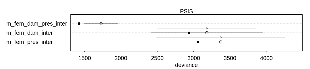
Ignoring the known outliers, PSIS believes the full interaction model performs best:

iplot(function() {
  plot(compare(m_fem_dam_pres_inter, m_fem_pres_inter, m_fem_dam_inter, func=PSIS))
}, ar=4.5)

Some Pareto k values are very high (>1). Set pointwise=TRUE to inspect individual points.

Some Pareto k values are very high (>1). Set pointwise=TRUE to inspect individual points.

Some Pareto k values are very high (>1). Set pointwise=TRUE to inspect individual points.

12H4. In the original hurricanes paper, storm damage (damage_norm) was used directly. This assumption implies that mortality increases exponentially with a linear increase in storm strength, because a Poisson regression uses a log link. So it’s worth exploring an alternative hypothesis: that the logarithm of storm strength is what matters. Explore this by using the logarithm of damage_norm as a predictor. Using the best model structure from the previous problem, compare a model that uses log(damage_norm) to a model that uses damage_norm directly. Compare their PSIS/WAIC values as well as their implied predictions. What do you conclude?

Answer We’ll use the full interaction model as our baseline, though it probably doesn’t matter which model we start from.

data(Hurricanes)
hur <- Hurricanes
hur$index = 1:92
hur$StdFem = standardize(hur$femininity)
hur$StdDam = standardize(hur$damage_norm)
hur$StdLogDam = standardize(log(hur$damage_norm))
hur$StdPres = standardize(hur$min_pressure)

hur_dat = list(
  Deaths = hur$deaths,
  StdFem = hur$StdFem,
  StdPres = hur$StdPres,
  StdDam = hur$StdDam
)

m_fem_dam_pres_inter <- quap(
  alist(
    Deaths ~ dpois(lambda),
    log(lambda) <- a + bFem * StdFem + bPres * StdPres + bDam * StdDam +
        bFemPresInter * StdFem * StdPres +
        bFemDamInter * StdFem * StdDam +
        bDamPresInter * StdDam * StdPres +
        bFDPInter * StdPres * StdDam * StdPres,
    a ~ dnorm(3, 0.5),
    bFem ~ dnorm(0, 1.0),
    bDam ~ dnorm(0, 1.0),
    bPres ~ dnorm(0, 1.0),
    bFemPresInter ~ dnorm(0, 0.4),
    bFemDamInter ~ dnorm(0, 0.4),
    bDamPresInter ~ dnorm(0, 0.4),
    bFDPInter ~ dnorm(0, 0.4)
  ),
  data = hur_dat
)

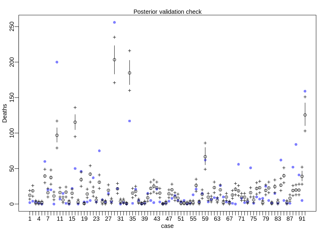
First we’ll run postcheck on the baseline model. Notice there is more dispersion than in the plain old Poisson model in 12H1:

iplot(function() {
  result <- postcheck(m_fem_dam_pres_inter, window=92)
  display_markdown("The raw data:")
  display(result)
})

hur_dat = list(
  Deaths = hur$deaths,
  StdFem = hur$StdFem,
  StdPres = hur$StdPres,
  StdLogDam = hur$StdLogDam
)

m_fem_logdam_pres_inter <- quap(
  alist(
    Deaths ~ dpois(lambda),
    log(lambda) <- a + bFem * StdFem + bPres * StdPres + bDam * StdLogDam +
        bFemPresInter * StdFem * StdPres +
        bFemDamInter * StdFem * StdLogDam +
        bDamPresInter * StdLogDam * StdPres +
        bFDPInter * StdPres * StdLogDam * StdPres,
    a ~ dnorm(3, 0.5),
    bFem ~ dnorm(0, 1.0),
    bDam ~ dnorm(0, 1.0),
    bPres ~ dnorm(0, 1.0),
    bFemPresInter ~ dnorm(0, 0.4),
    bFemDamInter ~ dnorm(0, 0.4),
    bDamPresInter ~ dnorm(0, 0.4),
    bFDPInter ~ dnorm(0, 0.4)
  ),
  data = hur_dat
)

The raw data:

$mean

1. 12.4192462885702
2. 18.5938168455421
3. 2.11381194508373
4. 1.77493954809473
5. 2.06508536687668
6. 39.4690667431158
7. 15.9610663893155
8. 37.358298332016
9. 11.3212801161669
10. 96.8666494831281
11. 16.2604276543812
12. 5.69564845261434
13. 16.8378743556131
14. 2.48682003620383
15. 15.2026808132042
16. 115.329975983529
17. 2.86569503514338
18. 34.4103632635181
19. 0.858249074601839
20. 14.1553490927226
21. 42.1341677686966
22. 17.2845656286884
23. 5.31305551387514
24. 30.7520944493205
25. 3.0837990192428
26. 2.48299529863905
27. 19.392170532057
28. 4.41411579164916
29. 203.384909416927
30. 21.504460642179
31. 3.7775803550042
32. 3.66808922049433
33. 0.910404527206778
34. 184.758064484002
35. 15.4002185551508
36. 17.9602111705932
37. 3.43535493602018
38. 0.82149797513125
39. 1.88977382488604
40. 8.87356128718296
41. 22.0901686916238
42. 25.2305705523166
43. 22.8483178647742
44. 15.4562893566688
45. 0.314647353158313
46. 1.75574042405943
47. 14.4320375051793
48. 20.0984933373014
49. 10.0849844222571
50. 8.29586575764401
51. 1.34149367017358
52. 1.28626217978254
53. 0.923591644163742
54. 2.23901284894469
55. 2.0416393055465
56. 26.2255624651538
57. 2.56590615956333
58. 13.8000154129816
59. 66.6899024324415
60. 9.76544195918975
61. 6.49516889581563
62. 23.198571097516
63. 5.28000404637473
64. 20.0148275741584
65. 2.33439640074048
66. 9.90300242282889
67. 1.7537386186061
68. 12.7469121252857
69. 20.8265191297282
70. 18.5405774511215
71. 9.72158475950537
72. 9.76524130280055
73. 3.46925119527546
74. 16.0444508846542
75. 5.8631354723675
76. 21.9122731810267
77. 23.0232995511413
78. 2.12003366427668
79. 19.1718685965319
80. 22.6813508455968
81. 1.37381187319183
82. 24.5510734365911
83. 2.68041577016984
84. 26.5396233012641
85. 39.8759313082704
86. 2.0679848610754
87. 8.08639310904994
88. 19.0363742456932
89. 19.7655928225731
90. 19.6766678257971
91. 39.04416705125
92. 125.520453680288

$PI

A matrix: 2 × 92 of type dbl

5%	11.70273	16.68520	1.759826	1.509584	1.797090	37.32644	15.03229	34.91078	10.57674	87.09672	⋯	2.347731	24.34544	37.31906	1.655340	7.358798	17.08223	17.76707	18.50674	32.38596	110.3816
94%	13.16521	20.59954	2.546389	2.081431	2.374178	41.58615	16.85816	39.80710	12.07033	107.53285	⋯	3.058250	28.75276	42.51885	2.554984	8.830958	21.07172	21.80052	20.90788	46.59840	142.5699

$outPI

A matrix: 2 × 92 of type dbl

5%	7	11	0	0	0.000	30	10	27.945	6	79	⋯	0	19	30.000	0	4	12	13.000	13	28.000	103
94%	19	26	5	4	4.055	49	22	48.000	17	117	⋯	6	36	51.055	5	13	26	27.055	28	52.055	151

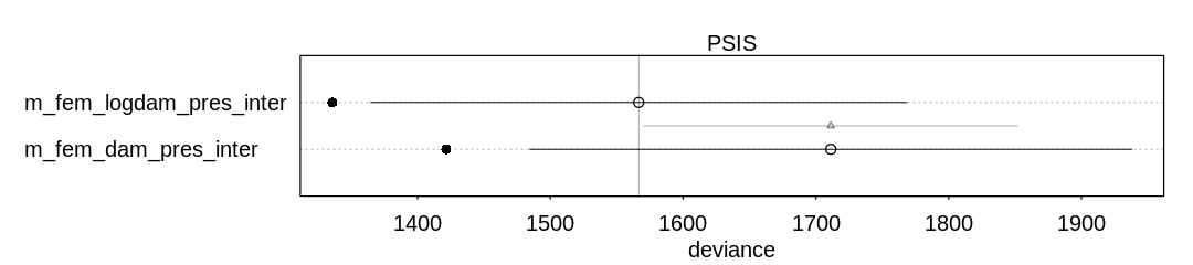
Ignoring the known outliers, comparing the models using PSIS, it appears the log(damage) model improves performance:

iplot(function() {
  plot(compare(m_fem_dam_pres_inter, m_fem_logdam_pres_inter, func=PSIS))
}, ar=4.5)

Some Pareto k values are very high (>1). Set pointwise=TRUE to inspect individual points.

Some Pareto k values are very high (>1). Set pointwise=TRUE to inspect individual points.

Run postcheck to visualize how much the model has changed on the outcome scale:

iplot(function() {
  result <- postcheck(m_fem_logdam_pres_inter, window=92)
  display_markdown("The raw data:")
  display(result)
})

The raw data:

$mean

1. 10.8699882836877
2. 16.2595681620299
3. 2.67255400951333
4. 0.324891055351021
5. 0.136794243571386
6. 41.0238249932624
7. 14.2206464899141
8. 49.9349468125643
9. 11.9320898678004
10. 154.499154480515
11. 20.5619727279893
12. 12.2148037384162
13. 4.4561389708142
14. 3.19519090024716
15. 4.50855930854229
16. 114.29724808675
17. 0.399705113340796
18. 45.2297046566204
19. 1.39761631106256
20. 26.8534972701785
21. 49.3207414632433
22. 12.6381635360833
23. 6.49466550321014
24. 36.1755561834113
25. 6.11465018583331
26. 0.988682407787108
27. 17.1613394443972
28. 6.69589713527632
29. 226.252793873048
30. 21.1241232209717
31. 3.07289094570769
32. 5.15026540733052
33. 0.832841989107325
34. 116.526910474906
35. 8.02121391702632
36. 20.756373368377
37. 4.27972358733588
38. 0.339424235355401
39. 2.15575129089143
40. 17.5665174746855
41. 19.4286826354081
42. 12.3566344076102
43. 33.532691484247
44. 3.85241425339933
45. 0.989993520191923
46. 3.27361461134978
47. 17.5895153295144
48. 12.8045063246198
49. 21.9652390357988
50. 9.03333226982972
51. 0.0193755906404282
52. 1.05886140918945
53. 0.0280480135459265
54. 0.0432815209135604
55. 2.21005348131204
56. 27.2597115785741
57. 4.89900537748048
58. 16.6009046234761
59. 82.6953189366748
60. 1.59268707136014
61. 12.4127603882858
62. 21.7426511119712
63. 6.3025973303236
64. 22.3686319891363
65. 4.3810954541357
66. 10.4123953524991
67. 3.45049157776192
68. 17.534453890374
69. 6.39968459072767
70. 18.1958495648466
71. 9.53385569354962
72. 8.27301885619899
73. 2.35454398034847
74. 18.9537906368423
75. 0.78951448157749
76. 23.6402882413444
77. 28.3081191196519
78. 3.51651372895571
79. 18.906859578512
80. 25.6698728834182
81. 2.07834564607815
82. 13.1695536352315
83. 0.824403690257513
84. 29.7669102790378
85. 43.0102158772508
86. 1.61453240811467
87. 7.97032785414566
88. 15.5282386088827
89. 20.7863785281744
90. 22.0236036269154
91. 31.6724471286218
92. 87.3912071579769

$PI

A matrix: 2 × 92 of type dbl

5%	10.10567	14.67018	2.150698	0.2387359	0.09846129	38.75203	13.26998	46.65318	11.14271	138.5229	⋯	0.6540991	27.78764	40.18345	1.192299	7.169494	13.90945	18.80923	20.68352	26.04830	79.13909
94%	11.64052	17.90678	3.232551	0.4271335	0.18349747	43.48464	15.25742	53.38582	12.77133	170.8846	⋯	1.0130670	32.00657	45.90527	2.135289	8.794958	17.12137	22.80798	23.46071	37.90813	95.99470

$outPI

A matrix: 2 × 92 of type dbl

5%	6	10	0	0	0	31	8	38	7	130	⋯	0.000	21	33	0	4	9	13	15	21	69
94%	16	23	6	1	1	52	20	62	18	181	⋯	2.055	39	54	4	13	22	28	30	42	104

12H5. One hypothesis from developmental psychology, usually attributed to Carol Gilligan, proposes that women and men have different average tendencies in moral reasoning. Like most hypotheses in social psychology, it is merely descriptive, not causal. The notion is that women are more concerned with care (avoiding harm), while men are more concerned with justice and rights. Evaluate this hypothesis, using the Trolley data, supposing that contact provides a proxy for physical harm. Are women more or less bothered by contact than are men, in these data? Figure out the model(s) that is needed to address this question.

Answer. The head of the Trolley data.frame:

data(Trolley)
d <- Trolley
display(head(Trolley))

A data.frame: 6 × 12

	case	response	order	id	age	male	edu	action	intention	contact	story	action2
	<fct>	<int>	<int>	<fct>	<int>	<int>	<fct>	<int>	<int>	<int>	<fct>	<int>
1	cfaqu	4	2	96;434	14	0	Middle School	0	0	1	aqu	1
2	cfbur	3	31	96;434	14	0	Middle School	0	0	1	bur	1
3	cfrub	4	16	96;434	14	0	Middle School	0	0	1	rub	1
4	cibox	3	32	96;434	14	0	Middle School	0	1	1	box	1
5	cibur	3	4	96;434	14	0	Middle School	0	1	1	bur	1
6	cispe	3	9	96;434	14	0	Middle School	0	1	1	spe	1

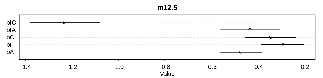
We’ll start from model m12.5 in the text, converting bC and bIC to index variables based on gender. Before doing the conversion, lets reproduce the precis summary for m12.5 in the text:

dat <- list(
  R = d$response,
  A = d$action,
  I = d$intention,
  C = d$contact
)
m12.5 <- ulam(
  alist(
    R ~ dordlogit(phi, cutpoints),
    phi <- bA * A + bC * C + BI * I,
    BI <- bI + bIA * A + bIC * C,
    c(bA, bI, bC, bIA, bIC) ~ dnorm(0, 0.5),
    cutpoints ~ dnorm(0, 1.5)
  ),
  data = dat, chains = 4, cores = min(detectCores(), 4), log_lik=TRUE
)

iplot(function() {
  plot(precis(m12.5), main="m12.5")
}, ar=4)

dat <- list(
  R = d$response,
  A = d$action,
  I = d$intention,
  C = d$contact,
  gid = ifelse(d$male == 1, 2, 1)
)
m_trolley_care <- ulam(
  alist(
    R ~ dordlogit(phi, cutpoints),
    phi <- bA * A + bC[gid] * C + BI * I,
    BI <- bI + bIA * A + bIC[gid] * C,
    c(bA, bI, bIA) ~ dnorm(0, 0.5),
    bC[gid] ~ dnorm(0, 0.5),
    bIC[gid] ~ dnorm(0, 0.5),
    cutpoints ~ dnorm(0, 1.5)
  ),
  data = dat, chains = 4, cores = min(detectCores(), 4), log_lik=TRUE
)
flush.console()

6 vector or matrix parameters hidden. Use depth=2 to show them.

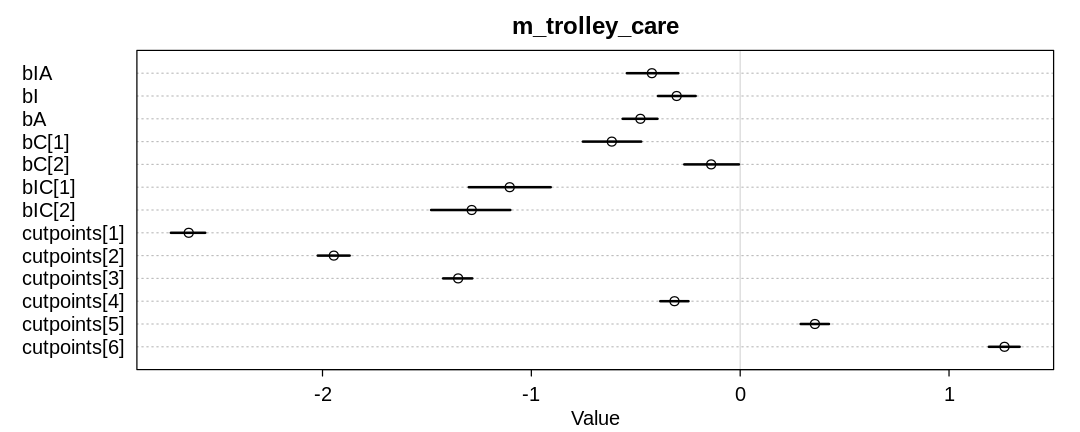
The following plot shows the same precis summary after converting bC and bIC to index variables based on gender. It appears women disapprove of contact more than men from this data and model, lending some support to the theory:

iplot(function() {
  plot(precis(m_trolley_care, depth=2), main="m_trolley_care")
}, ar=2.5)

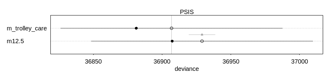
Comparing the models using PSIS, to check for overfitting or outliers:

iplot(function() {
  plot(compare(m12.5, m_trolley_care, func=PSIS))
}, ar=4.5)

12H6. The data in data(Fish) are records of visits to a national park. See ?Fish for details. The question of interest is how many fish an average visitor takes per hour, when fishing. The problem is that not everyone tried to fish, so the fish_caught numbers are zero-inflated. As with the monks example in the chapter, there is a process that determines who is fishing (working) and another process that determines fish per hour (manuscripts per day), conditional on fishing (working). We want to model both. Otherwise we’ll end up with an underestimate of rate of fish extraction from the park.

You will model these data using zero-inflated Poisson GLMs. Predict fish_caught as a function of any of the other variables you think are relevant. One thing you must do, however, is use a proper Poisson offset/exposure in the Poisson portion of the zero-inflated model. Then use the hours variable to construct the offset. This will adjust the model for the differing amount of time individuals spent in the park.

Answer. The short documentation on Fish:

display(help(Fish))

data(Fish)

Fish {rethinking}

R Documentation

Fishing data

Description

Fishing data from visitors to a national park.

Usage

data(Fish)

Format

1. fish_caught : Number of fish caught during visit

2. livebait : Whether or not group used livebait to fish

3. camper : Whether or not group had a camper

4. persons : Number of adults in group

5. child : Number of children in group

6. hours : Number of hours group spent in park

---

[Package rethinking version 2.13 ]

The head of Fish:

display(head(Fish))

A data.frame: 6 × 6

	fish_caught	livebait	camper	persons	child	hours
	<int>	<int>	<int>	<int>	<int>	<dbl>
1	0	0	0	1	0	21.124
2	0	1	1	1	0	5.732
3	0	1	0	1	0	1.323
4	0	1	1	2	1	0.548
5	1	1	0	1	0	1.695
6	0	1	1	4	2	0.493

Notice several outliers in the full dataframe (not represented in head):

display(summary(Fish))

  fish_caught         livebait         camper         persons     
 Min.   :  0.000   Min.   :0.000   Min.   :0.000   Min.   :1.000  
 1st Qu.:  0.000   1st Qu.:1.000   1st Qu.:0.000   1st Qu.:2.000  
 Median :  0.000   Median :1.000   Median :1.000   Median :2.000  
 Mean   :  3.296   Mean   :0.864   Mean   :0.588   Mean   :2.528  
 3rd Qu.:  2.000   3rd Qu.:1.000   3rd Qu.:1.000   3rd Qu.:4.000  
 Max.   :149.000   Max.   :1.000   Max.   :1.000   Max.   :4.000  
     child           hours        
 Min.   :0.000   Min.   : 0.0040  
 1st Qu.:0.000   1st Qu.: 0.2865  
 Median :0.000   Median : 1.8315  
 Mean   :0.684   Mean   : 5.5260  
 3rd Qu.:1.000   3rd Qu.: 7.3427  
 Max.   :3.000   Max.   :71.0360  

One complication introduced by the question and data is how to infer fish per ‘average visitor’ when every observation includes several visitors, both adults and children. This solution disregards children, assuming any fishing they do is offset by the time they take away from fishing. Addressing persons can be done the same way we address hours, by treating it as an exposure. That is: $\( \begin{align} log \left(\frac{fish}{person \cdot hour}\right) & = log(fish) - log(person \cdot hour) \\ & = log(fish) - log(person) - log(hour) \end{align} \)$

fish_dat <- list(
  FishCaught = Fish$fish_caught,
  LogPersonsInGroup = log(Fish$persons),
  LogHours = log(Fish$hours)
)

m_fish <- ulam(
  alist(
    FishCaught ~ dzipois(p, fish_per_person_hour),
    log(fish_per_person_hour) <- LogPersonsInGroup + LogHours + al,
    logit(p) <- ap,
    ap ~ dnorm(-0.5, 1),
    al ~ dnorm(1, 2)
  ), data = fish_dat, chains = 4
)
flush.console()

SAMPLING FOR MODEL '1a5d1436509eaa3c57b3600d89299fd9' NOW (CHAIN 1).
Chain 1: 
Chain 1: Gradient evaluation took 0.00012 seconds
Chain 1: 1000 transitions using 10 leapfrog steps per transition would take 1.2 seconds.
Chain 1: Adjust your expectations accordingly!
Chain 1: 
Chain 1: 
Chain 1: Iteration:   1 / 1000 [  0%]  (Warmup)
Chain 1: Iteration: 100 / 1000 [ 10%]  (Warmup)
Chain 1: Iteration: 200 / 1000 [ 20%]  (Warmup)
Chain 1: Iteration: 300 / 1000 [ 30%]  (Warmup)
Chain 1: Iteration: 400 / 1000 [ 40%]  (Warmup)
Chain 1: Iteration: 500 / 1000 [ 50%]  (Warmup)
Chain 1: Iteration: 501 / 1000 [ 50%]  (Sampling)
Chain 1: Iteration: 600 / 1000 [ 60%]  (Sampling)
Chain 1: Iteration: 700 / 1000 [ 70%]  (Sampling)
Chain 1: Iteration: 800 / 1000 [ 80%]  (Sampling)
Chain 1: Iteration: 900 / 1000 [ 90%]  (Sampling)
Chain 1: Iteration: 1000 / 1000 [100%]  (Sampling)
Chain 1: 
Chain 1:  Elapsed Time: 0.427317 seconds (Warm-up)
Chain 1:                0.288993 seconds (Sampling)
Chain 1:                0.71631 seconds (Total)
Chain 1: 

SAMPLING FOR MODEL '1a5d1436509eaa3c57b3600d89299fd9' NOW (CHAIN 2).
Chain 2: 
Chain 2: Gradient evaluation took 9e-05 seconds
Chain 2: 1000 transitions using 10 leapfrog steps per transition would take 0.9 seconds.
Chain 2: Adjust your expectations accordingly!
Chain 2: 
Chain 2: 
Chain 2: Iteration:   1 / 1000 [  0%]  (Warmup)
Chain 2: Iteration: 100 / 1000 [ 10%]  (Warmup)
Chain 2: Iteration: 200 / 1000 [ 20%]  (Warmup)
Chain 2: Iteration: 300 / 1000 [ 30%]  (Warmup)
Chain 2: Iteration: 400 / 1000 [ 40%]  (Warmup)
Chain 2: Iteration: 500 / 1000 [ 50%]  (Warmup)
Chain 2: Iteration: 501 / 1000 [ 50%]  (Sampling)
Chain 2: Iteration: 600 / 1000 [ 60%]  (Sampling)
Chain 2: Iteration: 700 / 1000 [ 70%]  (Sampling)
Chain 2: Iteration: 800 / 1000 [ 80%]  (Sampling)
Chain 2: Iteration: 900 / 1000 [ 90%]  (Sampling)
Chain 2: Iteration: 1000 / 1000 [100%]  (Sampling)
Chain 2: 
Chain 2:  Elapsed Time: 0.311079 seconds (Warm-up)
Chain 2:                0.256878 seconds (Sampling)
Chain 2:                0.567957 seconds (Total)
Chain 2: 

SAMPLING FOR MODEL '1a5d1436509eaa3c57b3600d89299fd9' NOW (CHAIN 3).
Chain 3: 
Chain 3: Gradient evaluation took 9.2e-05 seconds
Chain 3: 1000 transitions using 10 leapfrog steps per transition would take 0.92 seconds.
Chain 3: Adjust your expectations accordingly!
Chain 3: 
Chain 3: 
Chain 3: Iteration:   1 / 1000 [  0%]  (Warmup)
Chain 3: Iteration: 100 / 1000 [ 10%]  (Warmup)
Chain 3: Iteration: 200 / 1000 [ 20%]  (Warmup)
Chain 3: Iteration: 300 / 1000 [ 30%]  (Warmup)
Chain 3: Iteration: 400 / 1000 [ 40%]  (Warmup)
Chain 3: Iteration: 500 / 1000 [ 50%]  (Warmup)
Chain 3: Iteration: 501 / 1000 [ 50%]  (Sampling)
Chain 3: Iteration: 600 / 1000 [ 60%]  (Sampling)
Chain 3: Iteration: 700 / 1000 [ 70%]  (Sampling)
Chain 3: Iteration: 800 / 1000 [ 80%]  (Sampling)
Chain 3: Iteration: 900 / 1000 [ 90%]  (Sampling)
Chain 3: Iteration: 1000 / 1000 [100%]  (Sampling)
Chain 3: 
Chain 3:  Elapsed Time: 0.348026 seconds (Warm-up)
Chain 3:                0.290844 seconds (Sampling)
Chain 3:                0.63887 seconds (Total)
Chain 3: 

SAMPLING FOR MODEL '1a5d1436509eaa3c57b3600d89299fd9' NOW (CHAIN 4).
Chain 4: 
Chain 4: Gradient evaluation took 9.7e-05 seconds
Chain 4: 1000 transitions using 10 leapfrog steps per transition would take 0.97 seconds.
Chain 4: Adjust your expectations accordingly!
Chain 4: 
Chain 4: 
Chain 4: Iteration:   1 / 1000 [  0%]  (Warmup)
Chain 4: Iteration: 100 / 1000 [ 10%]  (Warmup)
Chain 4: Iteration: 200 / 1000 [ 20%]  (Warmup)
Chain 4: Iteration: 300 / 1000 [ 30%]  (Warmup)
Chain 4: Iteration: 400 / 1000 [ 40%]  (Warmup)
Chain 4: Iteration: 500 / 1000 [ 50%]  (Warmup)
Chain 4: Iteration: 501 / 1000 [ 50%]  (Sampling)
Chain 4: Iteration: 600 / 1000 [ 60%]  (Sampling)
Chain 4: Iteration: 700 / 1000 [ 70%]  (Sampling)
Chain 4: Iteration: 800 / 1000 [ 80%]  (Sampling)
Chain 4: Iteration: 900 / 1000 [ 90%]  (Sampling)
Chain 4: Iteration: 1000 / 1000 [100%]  (Sampling)
Chain 4: 
Chain 4:  Elapsed Time: 0.336802 seconds (Warm-up)
Chain 4:                0.291063 seconds (Sampling)
Chain 4:                0.627865 seconds (Total)
Chain 4: 

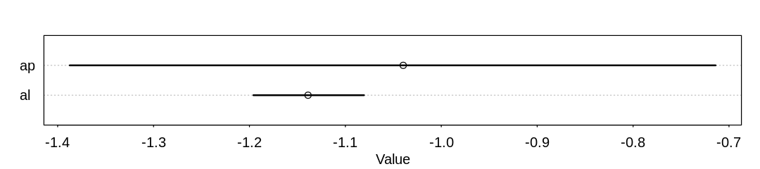
The precision of the parameters, which is rather hard to interpret. We can take from ap that most visitors who were a part of this survey chose to fish. That is, the probability of not fishing looks solidly below 0.5, since ap is solidly negative and any score less than zero implies a probability of less than 0.5:

iplot(function() {
  plot(precis(m_fish))
}, ar=4.5)

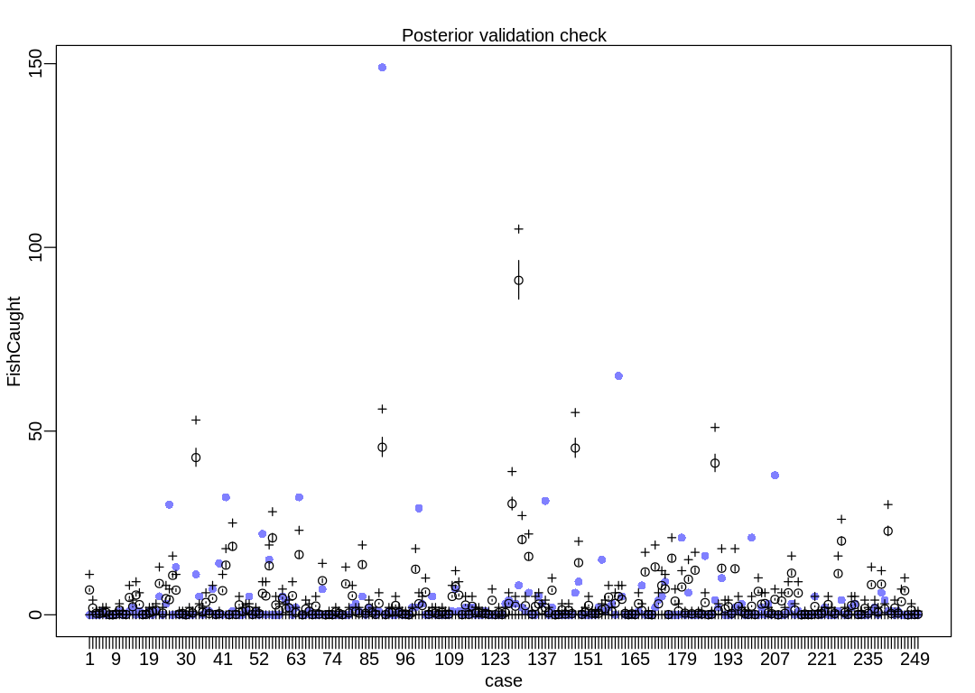
Finally, a posterior check. Despite the large uncertainty in ap the model is still surprised by outliers. An obvious alternative based on this chapter is a Gamma-Poisson, but this solution doesn’t pursue that.

iplot(function() {
  result <- postcheck(m_fish, window=250)
  display_markdown("The raw data:")
  display(result)
})

The raw data:

$mean

1. 6.76751586652509
2. 1.83636626334604
3. 0.423850761759738
4. 0.351126556983124
5. 0.543028753728462
6. 0.6317715058127
7. 0.031716723669096
8. 0.00512593513843976
9. 0.208561485945268
10. 1.29141528394067
11. 0.185815148768441
12. 0.0807334784304262
13. 4.7190640368261
14. 2.20287062574449
15. 5.37806707306176
16. 2.77345128084206
17. 0.0589482540920572
18. 0.136478023060959
19. 0.531815770613125
20. 0.85346820055022
21. 1.28404675217916
22. 8.50648936224078
23. 0.477352709767203
24. 4.4224005406889
25. 4.10299070737487
26. 10.7221748258314
27. 6.71625651514069
28. 0.221055952845215
29. 0.347282105629294
30. 0.0102518702768795
31. 0.805412558627347
32. 0.494973111805589
33. 42.7938695032643
34. 1.52881015503966
35. 0.693282727473977
36. 3.35876899946265
37. 0.337030235352414
38. 4.4480302163811
39. 0.0989946223611178
40. 0.293459786675676
41. 6.56792476707209
42. 13.5132465087118
43. 0.0442111905690429
44. 18.6173964228132
45. 0.0897038649226958
46. 2.70425115647313
47. 0.868205264073234
48. 1.51407309151664
49. 1.1994688223949
50. 0.0820149622150362
51. 0.851545974873305
52. 0.31588575290635
53. 5.83331418754444
54. 5.12657588033206
55. 13.3248683923741
56. 20.9330376216034
57. 2.67605851321171
58. 1.23759296498705
59. 4.52363775967309
60. 1.63357145443152
61. 1.89339229176119
62. 5.20730935876249
63. 0.595249217951317
64. 16.3786442510996
65. 0.0192222567691491
66. 1.58807878007787
67. 0.973927676303554
68. 0.0605501088228197
69. 2.39477282248982
70. 0.177485504168477
71. 9.29107780936822
72. 0.00897038649226958
73. 0.0858594135688659
74. 0.0384445135382982
75. 0.798684768758145
76. 0.41648222999823
77. 0.0413278520536706
78. 8.40781511082581
79. 0.504904611136316
80. 5.16566113576267
81. 0.850905232981
82. 0.465178613813408
83. 13.6593356601573
84. 0.409754440129028
85. 1.78702913763856
86. 0.555523220628409
87. 0.0999557351995753
88. 3.07908516347153
89. 45.610570861837
90. 0.0605501088228197
91. 0.650673391635697
92. 0.700330888289332
93. 2.54022123204305
94. 0.656119697720289
95. 0.226822629875959
96. 0.214328162976012
97. 0.0166592891999292
98. 0.622801119320431
99. 12.402200067455
100. 3.0294276668179
101. 2.51523229824316
102. 6.17867406749682
103. 0.161466956860852
104. 0.860195990419422
105. 0.456208227321139
106. 0.0884223811380858
107. 0.654838213935679
108. 0.140322474414788
109. 0.185815148768441
110. 4.99906824376337
111. 7.68922307860579
112. 5.36236889670029
113. 0.0509389804382451
114. 2.66676775577328
115. 0.108605750745692
116. 2.33678568123623
117. 0.497856450320962
118. 0.594608476059012
119. 0.411356294859791
120. 0.37387289415995
121. 0.126866894676384
122. 3.96010526539087
123. 0.0768890270765964
124. 0.574104735505253
125. 0.0666371567997169
126. 0.609986281474331
127. 3.08613332428689
128. 30.2356487850331
129. 2.34447458394388
130. 91.0314821235517
131. 20.4697812334669
132. 2.47838963943562
133. 15.8763026075325
134. 0.176844762276172
135. 2.28104113660569
136. 2.92306451269527
137. 1.32249126571746
138. 1.93856459516869
139. 0.545271350351529
140. 6.68421942052545
141. 0.0140963216307093
142. 0.0967520257380504
143. 1.34940242519427
144. 0.20760037310681
145. 1.18248916224882
146. 0.334467267783194
147. 45.3811852643918
148. 14.1812199314398
149. 0.122061330484097
150. 0.738134659935325
151. 2.54855087664302
152. 0.397259973229081
153. 0.373232152267645
154. 0.393415521875251
155. 1.40322474414788
156. 1.6249214388854
157. 4.80812715985649
158. 0.876534908673199
159. 3.12361672498673
160. 5.00419417890181
161. 4.21447979663594
162. 0.385406248221439
163. 0.0374834006998408
164. 0.261422692060428
165. 0.0551038027382274
166. 3.02173876411024
167. 1.18537250076419
168. 11.6640654075197
169. 0.0970723966842029
170. 0.0243481919075889
171. 13.0221178482601
172. 2.98073128300272
173. 7.96442172135078
174. 7.05328675049311
175. 0.0704816081535467
176. 15.3976684139807
177. 3.72719558753801
178. 1.03960372026481
179. 7.5684432319063
180. 0.453324888805766
181. 9.66302847785125
182. 0.278081981260357
183. 12.137573665933
184. 0.42801558405972
185. 0.199911470399151
186. 3.3139170670013
187. 0.0297944979921811
188. 0.172039198083884
189. 41.2714667671477
190. 1.16615024399505
191. 12.6665060980308
192. 1.63517330916228
193. 2.22529659197516
194. 0.370669184698425
195. 12.5290669621314
196. 2.32204861771321
197. 0.872370086373216
198. 0.347922847521599
199. 0.117896508184114
200. 2.34383384205158
201. 0.0800927365381213
202. 6.38435221492672
203. 2.9073663363338
204. 3.08260924387921
205. 0.538223189536175
206. 0.302750544114098
207. 4.20967423244365
208. 0.0128148378460994
209. 3.76980492337629
210. 0.414239633375163
211. 5.99349966062069
212. 11.3372870424441
213. 1.3080745731406
214. 5.9050772794826
215. 0.0115333540614895
216. 0.20760037310681
217. 0.0525408351690075
218. 0.0643945601766495
219. 2.27463371768264
220. 0.144807667660923
221. 0.352408040767733
222. 0.965918402649742
223. 2.78658648963431
224. 0.834886685673376
225. 0.329982074537059
226. 11.2084979220908
227. 20.083413872407
228. 0.59044365375903
229. 0.0913057196534582
230. 2.53413418406616
231. 2.72571600986534
232. 0.0820149622150361
233. 0.161466956860852
234. 1.74538091463874
235. 0.411997036752096
236. 8.19124435122674
237. 1.65503630782374
238. 0.685593824766318
239. 8.32612051955694
240. 1.62043624563927
241. 22.793752076857
242. 0.343437654275464
243. 1.84533664983831
244. 0.461334162459578
245. 3.58206754893093
246. 6.54774139746449
247. 0.00512593513843976
248. 1.26162078594849
249. 0.0720834628843091
250. 0.149292860907058

$PI

A matrix: 2 × 250 of type dbl

5%	6.388610	1.733550	0.4001198	0.3314674	0.5126252	0.5963993	0.02994094	0.004838939	0.1968843	1.219110	⋯	21.51755	0.3242089	1.742018	0.4355046	3.381511	6.181140	0.004838939	1.190984	0.06804759	0.1409341
94%	7.169384	1.945413	0.4490198	0.3719771	0.5752748	0.6692873	0.03360012	0.005430323	0.2209463	1.368102	⋯	24.14729	0.3638316	1.954916	0.4887291	3.794777	6.936559	0.005430323	1.336538	0.07636391	0.1581582

$outPI

A matrix: 2 × 250 of type dbl

5%	0	0	0	0	0	0	0	0	0	0	⋯	0	0	0	0	0	0.000	0	0	0	0
94%	11	4	1	1	2	2	0	0	1	3	⋯	30	1	4	1	7	10.055	0	3	1	1

12H7. In the trolley data — data(Trolley) — we saw how education level (modeled as an ordered category) is associated with responses. But is this association causal? One plausible confound is that education is also associated with age, through a causal process: People are older when they finish school than when they begin it. Reconsider the Trolley data in this light. Draw a DAG that represents hypothetical causal relationships among response, education, and age. Which statical model or models do you need to evaluate the causal influence of education on responses? Fit these models to the trolley data. What do you conclude about the causal relationships among these three variables?

ERROR:

Which statical [sic] model or models do you need

Answer. Consider the following DAGs. Implicit in this list of DAGs is that the response would never influence age or education. Because we already know that education is associated with the response, we also only include DAGs where Education and Response are d-connected.

A more difficult question is what arrows to allow between education and age. Getting older does not necessarily lead to more education, but education always leads to greater age. That is, someone could stop schooling at any point in their lives. This perspective implies Education should cause Age, because the choice to get a particular education is also a choice to get older before continuing with ‘real’ work.

The issue with allowing this arrow is it contradicts the following definition of Causal dependence from David Lewis:

An event E causally depends on C if, and only if, (i) if C had occurred, then E would have occurred, and (ii) if C had not occurred, then E would not have occurred.

Said another way, causality is almost always associated with the advancement of time. This is inherent in the definition of causality above, and in lists (see #4) such as the Bradford-Hill criteria. See also the definition of Causal inference. The Age covariate is confusingly a measurement of time. It is perhaps best to think of Age as a measurement of the potential to get education; greater Age indicates an individual is ‘richer’ in terms of time opportunity to get an education.

Said yet another way, age is not controllable. We will get older regardless of whether we get an education. Education on the other hand is clearly within our control. The issue seems to be that we require two things to get a particular educational degree: a personal commitment to do so and an investment of our time. We talk about investing our time when in the end we are always forced to invest it in something; we can’t choose to stay in a frozen present.

Said yet another way, we should not confuse prediction and causal inference. Someone’s education may help us predict their age, but this does not imply the relationship is causal.

Described as a rule for DAGs, indirect measures of time (like Age) can only have arrows pointing out of them. A convenient side effect of this rule is that to get the total causal effect of a variable like Age there should never be any back door paths to close.

Do these rules contradict general relativity? If there was a variable for how fast or far someone had traveled in their life (e.g. if they were an astronaut) couldn’t that cause a change in their Age? Perhaps in this extra special case you’d need to define a standardized time that all other time measurements were made relative to.

This perspective leads to other questions. Age does not necessarily indicate the level of education we will eventually achieve. Are people who had a healthy upbringing, e.g. with more material resources, more or less likely to provide disapproving responses, and also more or less likely to get an education? There are plenty of possible confounds that could influence both eventual education level and response, such as temperament. Would a 14 year old who will eventually get a PhD answer the same way to these questions now and after they finish their PhD?

Practially speaking, based on the wording in the question and the last paragraph of section 12.4, it seems the author wanted readers to only consider that Age influences Education (not vice versa).

See also the next question, which adds a few more comments on this issue.

Conditional independencies, if any, are listed under each DAG.

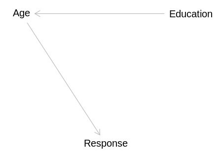
In this first model, education is a mediator between age and response:

library(dagitty)

age_dag <- dagitty('
dag {
    bb="0,0,1,1"
    Age [pos="0.4,0.2"]
    Education [pos="0.6,0.2"]
    Response [pos="0.5,0.3"]
    Age -> Education
    Education -> Response
}')
iplot(function() plot(age_dag), scale=10)
display(impliedConditionalIndependencies(age_dag))

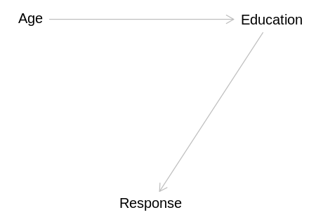
Age _||_ Rspn | Edct

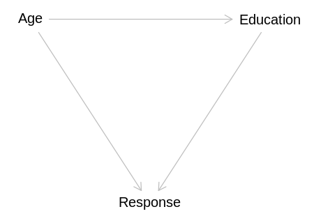
In this model, all variables are associated regardless of conditioning:

mediator_dag <- dagitty('
dag {
    bb="0,0,1,1"
    Age [pos="0.4,0.2"]
    Education [pos="0.6,0.2"]
    Response [pos="0.5,0.3"]
    Age -> Education
    Age -> Response
    Education -> Response
}')
iplot(function() plot(mediator_dag), scale=10)
display(impliedConditionalIndependencies(mediator_dag))

In this model, education has no direct causal effect on the response:

independent_dag <- dagitty('
dag {
    bb="0,0,1,1"
    Age [pos="0.4,0.2"]
    Education [pos="0.6,0.2"]
    Response [pos="0.5,0.3"]
    Age -> Education
    Age -> Response
}')
iplot(function() plot(independent_dag), scale=10)
display(impliedConditionalIndependencies(independent_dag))

Edct _||_ Rspn | Age

This answer will not consider this model because, as stated above, it seems more reasonable to assume that age leads to education than vice versa. Notice it has the same conditional independencies as the last model, and we could construct similar models where Education -> Age and with the same conditional independencies as the first and second models. Although that approach would work for this question, see comments in the next question.

independent_dag <- dagitty('
dag {
    bb="0,0,1,1"
    Age [pos="0.4,0.2"]
    Education [pos="0.6,0.2"]
    Response [pos="0.5,0.3"]
    Education -> Age
    Age -> Response
}')
iplot(function() plot(independent_dag), scale=10)
display(impliedConditionalIndependencies(independent_dag))

Edct _||_ Rspn | Age

To test which model is correct, we only need one more model beyond what we learned from m12.6 in the text: a model that includes age as a predictor. If we find that the education coefficient bE is near zero in this model, the third causal model is correct. If we find that the age coefficient is near zero, the first causal model is correct. If both coefficients are non-zero, we can infer the second causal model is correct. Of course, all causal inferences are limited by the variables we are considering.

data(Trolley)
d <- Trolley

edu_levels <- c(6, 1, 8, 4, 7, 2, 5, 3)
d$edu_new <- edu_levels[d$edu]

dat <- list(
  R = d$response,
  action = d$action,
  intention = d$intention,
  contact = d$contact,
  E = as.integer(d$edu_new),
  StdAge = standardize(d$age),
  alpha = rep(2, 7)
)

m_trolley_age <- ulam(
  alist(
    R ~ ordered_logistic(phi, kappa),
    phi <- bE * sum(delta_j[1:E]) + bStdAge * StdAge + bA * action + bI * intention + bC * contact,
    kappa ~ normal(0, 1.5),
    c(bA, bI, bC, bE, bStdAge) ~ normal(0, 1),
    vector[8]:delta_j <<- append_row(0, delta),
    simplex[7]:delta ~ dirichlet(alpha)
  ),
  data = dat, chains = 4, cores = min(detectCores(), 4), iter=2000
)

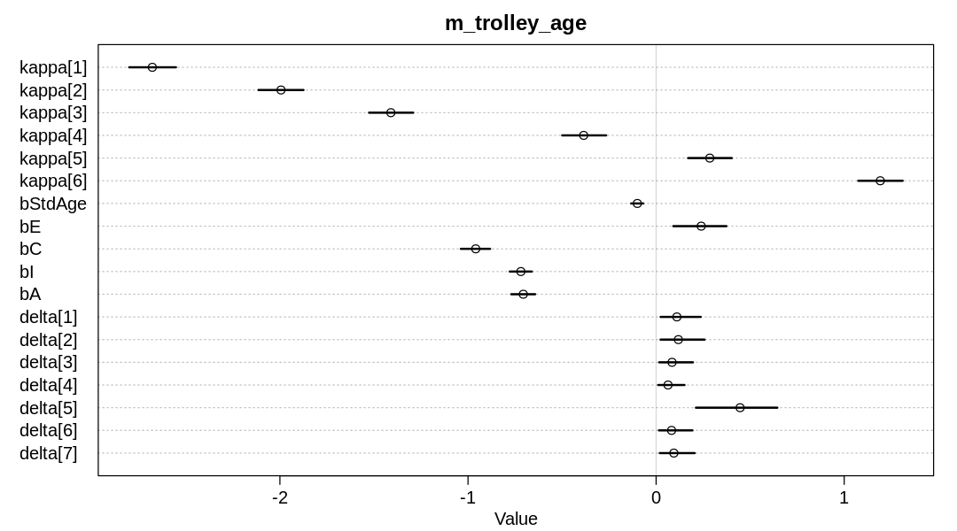
iplot(function() {
  plot(precis(m_trolley_age, depth=2), main="m_trolley_age")
}, ar=1.8)
display_markdown("Raw data (preceding plot):")
display(precis(m_trolley_age, depth = 2), mimetypes="text/plain")

Raw data (preceding plot):

         mean        sd         5.5%        94.5%       n_eff     Rhat4    
kappa[1] -2.67830561 0.08343011 -2.80122645 -2.55278302 1078.6704 1.0024045
kappa[2] -1.99419504 0.08108227 -2.11397697 -1.87468153 1028.9019 1.0025716
kappa[3] -1.41015518 0.07981220 -1.52607675 -1.29153444 1003.5752 1.0027147
kappa[4] -0.38516554 0.07943401 -0.49912643 -0.26571646 1009.6277 1.0031024
kappa[5]  0.28527392 0.07997250  0.17009254  0.40234439  988.9081 1.0032235
kappa[6]  1.19187995 0.08146554  1.07484372  1.31077185 1030.7310 1.0029348
bStdAge  -0.09980456 0.02057290 -0.13243610 -0.06778931 2478.8851 1.0011160
bE        0.23973082 0.09967973  0.09144668  0.37359848  824.1898 1.0039400
bC       -0.95887192 0.04860664 -1.03782058 -0.88270538 3987.0337 0.9993633
bI       -0.71895204 0.03683421 -0.77789181 -0.66061573 4279.5796 1.0002961
bA       -0.70615415 0.04017477 -0.77006368 -0.64310355 3974.8459 0.9997743
delta[1]  0.11041244 0.06987493  0.02386914  0.23702128 4110.5247 1.0002486
delta[2]  0.11840614 0.07534208  0.02369014  0.25798016 5122.1495 0.9994711
delta[3]  0.08474526 0.05982338  0.01655209  0.19596407 3165.8438 1.0014157
delta[4]  0.06340311 0.04964455  0.01127020  0.15086570 1929.8542 1.0011308
delta[5]  0.44650719 0.13548407  0.21163334  0.64445624 1373.2541 1.0020109
delta[6]  0.08217264 0.05801588  0.01511948  0.19316777 4390.0564 0.9994020
delta[7]  0.09435321 0.06108534  0.01951332  0.20496406 4283.7173 0.9999439

As implied in the text, it is not correct to causally infer the associated of education bE is negative based on m12.6. In this model, the association of education with response has reversed, becoming positive. Since the error bars on neither bStdAge or bE cross zero, we’ll infer for now that the second causal model above is correct.

12H8. Consider one more variable in the trolley data: Gender. Suppose that gender might influence education as well as response directly. Draw the DAG now that includes response, education, age, and gender. Using only the DAG, is it possible that the inferences from 12H7 above are confounded by gender? If so, define any additional models you need to infer the causal influence of education on response. What do you conclude?

Answer. First, lets consider a DAG that doesn’t work. In the following DAG we assume Education -> Age rather than that Age -> Gender:

incorrect_dag <- dagitty('
dag {
    bb="0,0,1,1"
    Education [pos="0.4,0.2"]
    Age [pos="0.6,0.2"]
    Response [pos="0.5,0.3"]
    Gender [pos="0.3,0.3"]
    Education -> Age
    Education -> Response
    Age -> Response
    Gender -> Education
    Gender -> Response
}')
iplot(function() plot(incorrect_dag), scale=10)
display(impliedConditionalIndependencies(incorrect_dag))

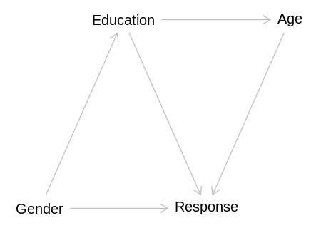
Age _||_ Gndr | Edct

With the additions implied by this question, this DAG implies that Gender will be able to predict Age without conditioning, which is not correct.

Instead, we’ll add this question’s covariate to the second model from the last question:

gender_dag <- dagitty('
dag {
    bb="0,0,1,1"
    Age [pos="0.4,0.2"]
    Education [pos="0.6,0.2"]
    Response [pos="0.5,0.3"]
    Gender [pos="0.7,0.3"]
    Age -> Education
    Education -> Response
    Age -> Response
    Gender -> Education
    Gender -> Response
}')
iplot(function() plot(gender_dag), scale=10)
display(impliedConditionalIndependencies(gender_dag))

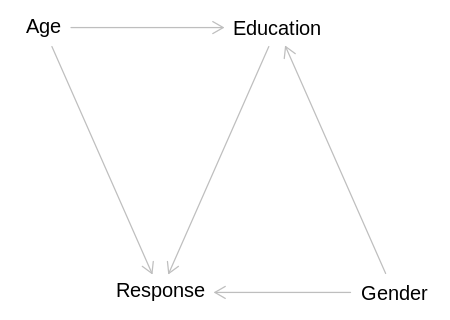
Age _||_ Gndr

This DAG implies Age will always be independent of Gender, which seems reasonable in this context, ignoring that females live slightly longer than males. To infer either the direct or total causal effect of Education on Response the required adjustment is to condition on both Age and Gender:

display(adjustmentSets(gender_dag, exposure="Education", outcome="Response", effect="total"))

{ Age, Gender }

We can do so by fitting a model that includes all three variables as predictors of Response:

data(Trolley)
d <- Trolley

edu_levels <- c(6, 1, 8, 4, 7, 2, 5, 3)
d$edu_new <- edu_levels[d$edu]

dat <- list(
  R = d$response,
  action = d$action,
  intention = d$intention,
  contact = d$contact,
  E = as.integer(d$edu_new),
  StdAge = standardize(d$age),
  gid = ifelse(d$male == 1, 2, 1),
  alpha = rep(2, 7)
)

# This fit takes more than three hours with 4 chains/cores.
m_trolley_gender <- ulam(
  alist(
    R ~ ordered_logistic(phi, kappa),
    phi <- bE * sum(delta_j[1:E]) + bStdAge * StdAge + bGender[gid]
        + bA * action + bI * intention + bC * contact,
    kappa ~ normal(0, 1.5),
    bGender[gid] ~ normal(0, 1),
    c(bA, bI, bC, bE, bStdAge) ~ normal(0, 1),
    vector[8]:delta_j <<- append_row(0, delta),
    simplex[7]:delta ~ dirichlet(alpha)
  ),
  data = dat, chains = 2, cores = min(detectCores(), 2), iter=1600
)
flush.console()

iplot(function() {
  plot(precis(m_trolley_gender, depth=2), main="m_trolley_gender")
}, ar=1.8)
display_markdown("Raw data (preceding plot):")
display(precis(m_trolley_gender, depth = 2), mimetypes="text/plain")

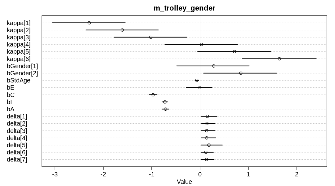
Raw data (preceding plot):

           mean         sd         5.5%        94.5%       n_eff     Rhat4    
kappa[1]   -2.291288958 0.46714983 -3.05260629 -1.54696264  659.4706 0.9999423
kappa[2]   -1.607263559 0.46604267 -2.36025842 -0.86161796  651.3348 0.9999119
kappa[3]   -1.017986406 0.46601190 -1.77572631 -0.27447415  646.3224 0.9999655
kappa[4]    0.027295827 0.46724972 -0.72466027  0.77361815  650.8136 0.9999874
kappa[5]    0.713412755 0.46689327 -0.04813372  1.46074243  646.8730 1.0000190
kappa[6]    1.640855013 0.46595949  0.87522556  2.40258796  656.7113 1.0000113
bGender[1]  0.281718757 0.47214155 -0.48282535  1.01670089  648.9819 1.0008279
bGender[2]  0.842675884 0.47292313  0.07431572  1.58122866  650.7906 1.0007947
bStdAge    -0.065964224 0.02168272 -0.10192004 -0.03280363  656.3598 1.0031312
bE         -0.002843373 0.17313847 -0.28393684  0.24594105  432.4367 1.0069854
bC         -0.971089462 0.05088699 -1.05192433 -0.89012013 1163.9056 1.0005626
bI         -0.727087854 0.03724670 -0.78542080 -0.66563698 1484.6136 1.0001663
bA         -0.714202313 0.04216100 -0.78006046 -0.64593394 1198.0312 1.0014116
delta[1]    0.151104519 0.10052852  0.03023021  0.34580260 1200.1489 0.9999488
delta[2]    0.142577365 0.08988162  0.03408959  0.30904329 1532.9985 0.9996467
delta[3]    0.136646640 0.09215948  0.02706038  0.30950045 1307.6900 1.0005605
delta[4]    0.135418403 0.09860457  0.02332306  0.32535805  891.6557 1.0019536
delta[5]    0.183354260 0.15339020  0.01686351  0.46168231  533.0076 1.0071922
delta[6]    0.119878490 0.07915463  0.02342631  0.27391009 1886.3322 0.9990988
delta[7]    0.131020323 0.08137387  0.02700134  0.27988752 1990.5208 1.0010292

At this point, education appears to have no causal effect on response. That is, the mean and HPDI of bE are near zero.