
Practice: Chp. 13#
source("iplot.R")
suppressPackageStartupMessages(library(rethinking))
13E1. Which of the following priors will produce more shrinkage in the estimates?
(a) \(\alpha_{tank} \sim Normal(0,1)\)
(b) \(\alpha_{tank} \sim Normal(0,2)\)
Answer. We could interpret this question in two ways. The first is that the author meant to write:
(a) \(\bar{\alpha} \sim Normal(0,1)\)
(b) \(\bar{\alpha} \sim Normal(0,2)\)
That is, interpretion #1 is that these are priors for the hyperparameter for the average of all tanks, with no new prior specified for the hyperparameter for the variability among tanks \(\sigma\).
The second interpretation is that the author is trying to express in shorthand new priors for both the \(\bar{\alpha}\) and \(\sigma\) priors, and only the expected value of these two priors, ignoring a standard deviation. To use the same terms as the chapter:
(a) \(\alpha_{tank} \sim Normal(\bar{\alpha},\sigma), \bar{\alpha} \sim Normal(0,?), \sigma \sim Exponential(1)\)
(b) \(\alpha_{tank} \sim Normal(\bar{\alpha},\sigma), \bar{\alpha} \sim Normal(0,?), \sigma \sim Exponential(\frac{1}{2})\)
Notice we decrease the \(\lambda\) parameter to the exponential distribution to increase the expected value.
Said another way, the first interpretation is that the author meant to specify this prior at the second level of the model, and the second interpretation is that the author meant to specify this prior at the first level. The first interpretation makes sense given this prior shows up directly in models in the chapter already, without much reinterpretation. The second interpretation is supported by the author’s choice of variable name (e.g. see the chapter and question 13M3). See also question 13M5.
In both interpretations, prior (a) will produce more shrinkage because it is more regularizing. It has a smaller standard deviation and therefore expects less variability.
13E2. Rewrite the following model as a multilevel model.
Answer. The focus of this chapter is on varying intercepts rather than varying effects (see the next chapter), so we’ll only convert the intercept:
13E3. Rewrite the following model as a multilevel model.
Answer. As in the last question, we’ll only convert the intercept:
13E4. Write a mathematical model formula for a Poisson regression with varying intercepts.
13E5. Write a mathematical model formula for a Poisson regression with two different kinds of varying intercepts, a cross-classified model.
13M1. Revisit the Reed frog survival data, data(reedfrogs), and add the predation and size
treatment variables to the varying intercept model. Consider models with either main effect alone,
both main effects, as well as a model including both and their interaction. Instead of focusing on
inferences about these two predictor variables, focus on the inferred variation across tanks.
Explain why it changes as it does across models.
ERROR. The predation predictor is actually labeled pred.
ERROR. The author duplicated this question in 13H4, without realizing he had moved it and primarily only changed wording.
Compare the second sentences:
Consider models with either main effect alone, both main effects, as well as a model including both and their interaction.
Consider models with either predictor alone, both predictors, as well as a model including their interaction.
One sentence only exists in 13H4:
What do you infer about the causal inference of these predictor variables?
Compare the last two sentences:
Instead of focusing on inferences about these two predictor variables, focus on the inferred variation across tanks. Explain why it changes as it does across models.
Also focus on the inferred variation across tanks (the \(\sigma\) across tanks). Explain why it changes as it does across models with different predictors included.
We could treat 13H4 as a separate question that expands on 13M1 by adding causal inference, but this answer will combine the two.
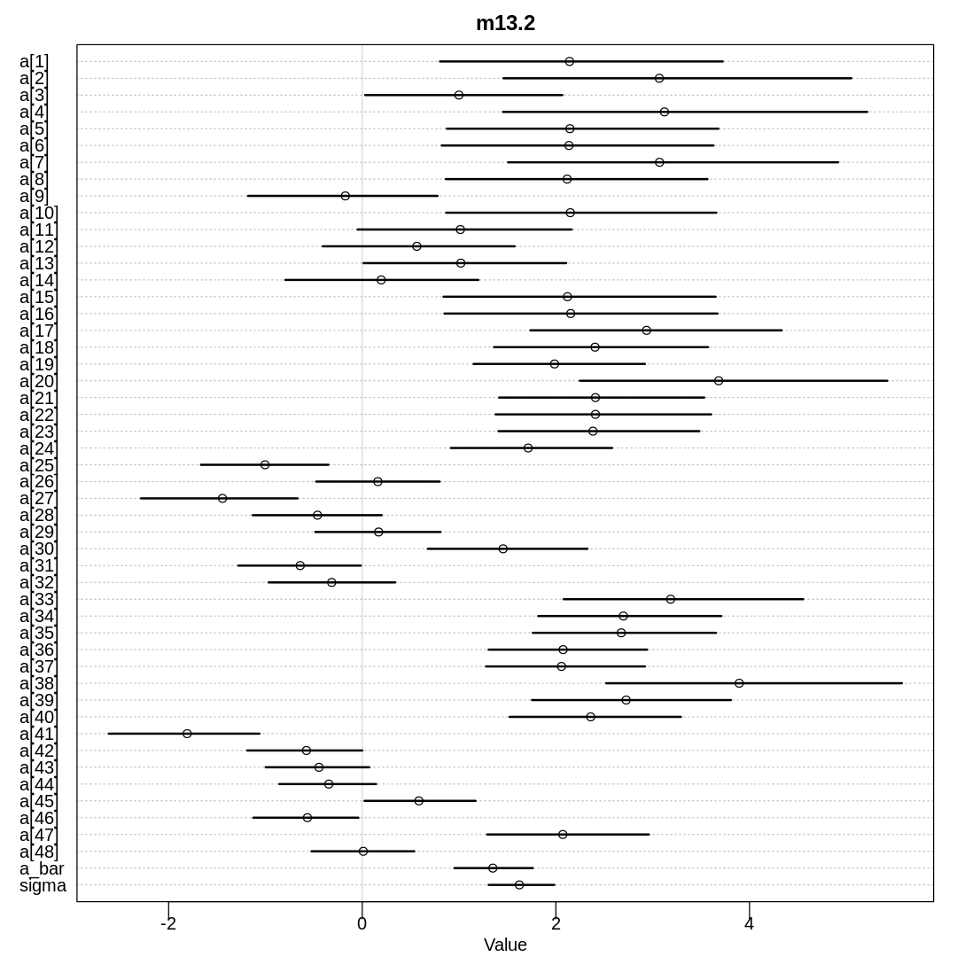
Answer. First, let’s reproduce results from model m13.2 in the chapter:
data(reedfrogs)
rf_df <- reedfrogs
rf_df$tank <- 1:nrow(rf_df)

rf_dat <- list(
  S = rf_df$surv,
  N = rf_df$density,
  tank = rf_df$tank
)

## R code 13.3
m13.2 <- ulam(
  alist(
    S ~ dbinom(N, p),
    logit(p) <- a[tank],
    a[tank] ~ dnorm(a_bar, sigma),
    a_bar ~ dnorm(0, 1.5),
    sigma ~ dexp(1)
  ),
  data = rf_dat, chains = 4, cores = 4, log_lik = TRUE
)

iplot(function() {
  plot(precis(m13.2, depth=2), main='m13.2')
}, ar=1.0)

Raw data (preceding plot):
display(precis(m13.2, depth = 2), mimetypes="text/plain")

rf_df$Predator <- as.integer(as.factor(rf_df$pred))
rf_df$Size <- as.integer(as.factor(rf_df$size))
rf_df$Treatment <- 1 + ifelse(rf_df$Predator == 1, 0, 1) + 2*ifelse(rf_df$Size == 1, 0, 1)
      mean         sd        5.5%         94.5%       n_eff    Rhat4
a[1]   2.140870552 0.8859526  0.804519773  3.62566247 2353.138 1.0010291
a[2]   3.063712215 1.1026424  1.518797394  4.93653182 2525.864 0.9996828
a[3]   0.988030759 0.6501472 -0.007850253  2.05339638 3770.161 1.0001676
a[4]   3.059445998 1.0953632  1.492975040  4.99029437 2512.501 0.9991452
a[5]   2.137361211 0.8835823  0.830563049  3.63390129 3578.324 0.9989542
a[6]   2.155645148 0.9120397  0.775677124  3.68057627 3839.725 0.9985621
a[7]   3.075375888 1.0828954  1.503543081  4.88250719 2608.287 0.9998512
a[8]   2.116734673 0.8383498  0.871596373  3.55196465 3303.001 0.9983033
a[9]  -0.167041461 0.5898447 -1.116855536  0.76347521 3783.739 0.9988444
a[10]  2.148970941 0.8771241  0.827365434  3.66932740 5534.857 0.9989499
a[11]  1.006415034 0.6678171 -0.012397076  2.08815029 3227.464 0.9990316
a[12]  0.565510764 0.6192286 -0.398704775  1.58486705 4826.174 1.0000180
a[13]  1.003919106 0.6749454 -0.061658610  2.14258077 4461.055 0.9985976
a[14]  0.198131086 0.6341755 -0.821541356  1.24364224 3643.883 0.9994165
a[15]  2.121903811 0.8893235  0.806022762  3.62297278 2719.969 1.0002527
a[16]  2.108712825 0.8140236  0.925250797  3.56708621 2858.796 0.9986126
a[17]  2.902203665 0.7841467  1.816014459  4.28888910 2600.156 0.9992230
a[18]  2.395064529 0.6942361  1.406794072  3.59130504 3956.609 1.0002657
a[19]  2.016295400 0.5949755  1.128505085  3.03695357 2936.907 0.9992657
a[20]  3.672251610 1.0160430  2.209785523  5.36019995 3128.385 1.0001016
a[21]  2.400173712 0.6653873  1.401848076  3.50284908 3699.696 1.0005130
a[22]  2.394330215 0.6339378  1.446961546  3.45487710 3203.959 0.9989266
a[23]  2.401877950 0.6441432  1.406323933  3.50286860 2642.005 0.9989273
a[24]  1.713757063 0.5190089  0.932277570  2.57072331 3878.162 0.9986886
a[25] -0.992097242 0.4317533 -1.688886130 -0.32855828 2942.442 0.9994747
a[26]  0.161420606 0.3825513 -0.462928025  0.78386327 4052.027 0.9985120
a[27] -1.417213902 0.4789801 -2.206584823 -0.69404456 3337.709 0.9991123
a[28] -0.464126916 0.4060543 -1.141359736  0.19802559 3680.799 0.9995168
a[29]  0.155839266 0.3996899 -0.470584650  0.81145649 6012.421 0.9985943
a[30]  1.455129784 0.4987695  0.688134703  2.29580848 3953.658 1.0000610
a[31] -0.645714440 0.4039465 -1.281935345 -0.00342412 3887.709 0.9986925
a[32] -0.311872075 0.4078103 -0.969318389  0.34083098 4056.769 0.9983916
a[33]  3.176435245 0.7606534  2.070428472  4.45912033 2752.091 0.9993933
a[34]  2.697554930 0.6152821  1.782205692  3.73042723 3559.540 0.9986566
a[35]  2.707437880 0.6351259  1.771433281  3.81797055 3795.629 0.9991654
a[36]  2.058356157 0.5302910  1.274204523  2.94312879 3982.459 0.9991647
a[37]  2.057286908 0.5056706  1.283005595  2.88463934 4221.378 0.9989490
a[38]  3.879500445 0.9280132  2.588616848  5.48244760 2584.128 0.9996489
a[39]  2.703061148 0.6441085  1.739697098  3.81203498 3081.946 1.0003448
a[40]  2.359251301 0.5780981  1.502286862  3.33415671 3786.215 0.9986930
a[41] -1.798051220 0.4652609 -2.573945840 -1.09635929 3546.866 0.9996111
a[42] -0.568695547 0.3616373 -1.167271560  0.01422360 4255.017 0.9992838
a[43] -0.455482934 0.3516919 -1.018578808  0.08420861 4514.875 0.9991946
a[44] -0.328346356 0.3290851 -0.854352985  0.19038827 4376.961 1.0000102
a[45]  0.586550069 0.3628149 -0.007393136  1.18375737 3934.524 0.9995949
a[46] -0.564929017 0.3360715 -1.107008057 -0.03729633 3235.905 1.0019583
a[47]  2.042860950 0.4985365  1.274979300  2.90080334 3716.675 0.9998204
a[48]  0.003818859 0.3451206 -0.549706577  0.56287288 3651.393 0.9993183
a_bar  1.341477329 0.2472076  0.942773123  1.74880023 2862.745 0.9994041
sigma  1.609156175 0.2043256  1.311751463  1.95342204 1701.388 1.0013158
The reedfrogs data.frame is small enough to show in its entirety. Notice several new preprocessed
variables (columns) this solution will introduce later as they are used in models:
display(rf_df)
| density | pred | size | surv | propsurv | tank | Predator | Size | Treatment |
|---|---|---|---|---|---|---|---|---|
| <int> | <fct> | <fct> | <int> | <dbl> | <int> | <int> | <int> | <dbl> |
| 10 | no | big | 9 | 0.9000000 | 1 | 1 | 1 | 1 |
| 10 | no | big | 10 | 1.0000000 | 2 | 1 | 1 | 1 |
| 10 | no | big | 7 | 0.7000000 | 3 | 1 | 1 | 1 |
| 10 | no | big | 10 | 1.0000000 | 4 | 1 | 1 | 1 |
| 10 | no | small | 9 | 0.9000000 | 5 | 1 | 2 | 3 |
| 10 | no | small | 9 | 0.9000000 | 6 | 1 | 2 | 3 |
| 10 | no | small | 10 | 1.0000000 | 7 | 1 | 2 | 3 |
| 10 | no | small | 9 | 0.9000000 | 8 | 1 | 2 | 3 |
| 10 | pred | big | 4 | 0.4000000 | 9 | 2 | 1 | 2 |
| 10 | pred | big | 9 | 0.9000000 | 10 | 2 | 1 | 2 |
| 10 | pred | big | 7 | 0.7000000 | 11 | 2 | 1 | 2 |
| 10 | pred | big | 6 | 0.6000000 | 12 | 2 | 1 | 2 |
| 10 | pred | small | 7 | 0.7000000 | 13 | 2 | 2 | 4 |
| 10 | pred | small | 5 | 0.5000000 | 14 | 2 | 2 | 4 |
| 10 | pred | small | 9 | 0.9000000 | 15 | 2 | 2 | 4 |
| 10 | pred | small | 9 | 0.9000000 | 16 | 2 | 2 | 4 |
| 25 | no | big | 24 | 0.9600000 | 17 | 1 | 1 | 1 |
| 25 | no | big | 23 | 0.9200000 | 18 | 1 | 1 | 1 |
| 25 | no | big | 22 | 0.8800000 | 19 | 1 | 1 | 1 |
| 25 | no | big | 25 | 1.0000000 | 20 | 1 | 1 | 1 |
| 25 | no | small | 23 | 0.9200000 | 21 | 1 | 2 | 3 |
| 25 | no | small | 23 | 0.9200000 | 22 | 1 | 2 | 3 |
| 25 | no | small | 23 | 0.9200000 | 23 | 1 | 2 | 3 |
| 25 | no | small | 21 | 0.8400000 | 24 | 1 | 2 | 3 |
| 25 | pred | big | 6 | 0.2400000 | 25 | 2 | 1 | 2 |
| 25 | pred | big | 13 | 0.5200000 | 26 | 2 | 1 | 2 |
| 25 | pred | big | 4 | 0.1600000 | 27 | 2 | 1 | 2 |
| 25 | pred | big | 9 | 0.3600000 | 28 | 2 | 1 | 2 |
| 25 | pred | small | 13 | 0.5200000 | 29 | 2 | 2 | 4 |
| 25 | pred | small | 20 | 0.8000000 | 30 | 2 | 2 | 4 |
| 25 | pred | small | 8 | 0.3200000 | 31 | 2 | 2 | 4 |
| 25 | pred | small | 10 | 0.4000000 | 32 | 2 | 2 | 4 |
| 35 | no | big | 34 | 0.9714286 | 33 | 1 | 1 | 1 |
| 35 | no | big | 33 | 0.9428571 | 34 | 1 | 1 | 1 |
| 35 | no | big | 33 | 0.9428571 | 35 | 1 | 1 | 1 |
| 35 | no | big | 31 | 0.8857143 | 36 | 1 | 1 | 1 |
| 35 | no | small | 31 | 0.8857143 | 37 | 1 | 2 | 3 |
| 35 | no | small | 35 | 1.0000000 | 38 | 1 | 2 | 3 |
| 35 | no | small | 33 | 0.9428571 | 39 | 1 | 2 | 3 |
| 35 | no | small | 32 | 0.9142857 | 40 | 1 | 2 | 3 |
| 35 | pred | big | 4 | 0.1142857 | 41 | 2 | 1 | 2 |
| 35 | pred | big | 12 | 0.3428571 | 42 | 2 | 1 | 2 |
| 35 | pred | big | 13 | 0.3714286 | 43 | 2 | 1 | 2 |
| 35 | pred | big | 14 | 0.4000000 | 44 | 2 | 1 | 2 |
| 35 | pred | small | 22 | 0.6285714 | 45 | 2 | 2 | 4 |
| 35 | pred | small | 12 | 0.3428571 | 46 | 2 | 2 | 4 |
| 35 | pred | small | 31 | 0.8857143 | 47 | 2 | 2 | 4 |
| 35 | pred | small | 17 | 0.4857143 | 48 | 2 | 2 | 4 |
The help is also short:
display(help(reedfrogs))
| reedfrogs {rethinking} | R Documentation |
Data on reed frog predation experiments
Description
Data on lab experiments on the density- and size-dependent predation rate of an African reed frog, Hyperolius spinigularis, from Vonesh and Bolker 2005
Usage
data(reedfrogs)
Format
Various data with variables:
densityinitial tadpole density (number of tadpoles in a 1.2 x 0.8 x 0.4 m tank) [experiment 1]
predfactor: predators present or absent [experiment 1]
sizefactor: big or small tadpoles [experiment 1]
survnumber surviving
propsurvproportion surviving (=surv/density) [experiment 1]
Source
Vonesh and Bolker (2005) Compensatory larval responses shift trade-offs associated with predator-induced hatching plasticity. Ecology 86:1580-1591
Examples
data(reedfrogs)
boxplot(propsurv~size*density*pred,data=reedfrogs)
Our first model will add the pred predictor on only the first level:
Seeing as this is a chapter on multilevel models, and it’s generally advisable to consider a multilevel model when we have exchangeable index variables, should we add a second level of parameters for this predictor? In other words:
The problem with this model is that there are only 2 (rather than 48) clusters for us to learn from, that is, we are adding one second-level parameter to go with only two first-level parameters. Said another way, do our clusters have anything to learn from each other? It may help to not forget about the last tank of tadpoles when learning about a new one, or the last chimp when learning about a new one, but in this case there is only one other pool to learn from: either all predator pools, or all non-predator pools.
We could try to remember what we learned about one predator pool when moving to another predator
pool. In this approach, we would learn one \(\bar{\alpha}\) and one \(\sigma\) for the predator pools,
and one \(\bar{\alpha}\) and one \(\sigma\) for the non-predator pools. Presumably this would require
reindexing predator and non-predator pools from 1..24. The original model from the chapter already
has an intercept for individual pools this approach would likely not differ significantly from, so
we will avoid these complications and only add pred on the first level.
Now let’s fit our new model, with a pred predictor on the first level. This model struggles to fit
as provided above. To avoid Stan warnings about RHat, Bulk ESS, and Tail ESS, we’re actually going
to fit a model with a different \(\bar{\alpha}\) prior than the one proposed above:
See more comments on this tight \(\bar{\alpha}\) prior below.
rf_dat <- list(
  S = rf_df$surv,
  N = rf_df$density,
  tank = rf_df$tank,
  Predator = rf_df$Predator
)

m_rf_pred_orig <- ulam(
  alist(
    S ~ dbinom(N, p),
    logit(p) <- a[tank] + bPredator[Predator],
    a[tank] ~ dnorm(a_bar, sigma),
    a_bar ~ dnorm(0, 0.1),
    sigma ~ dexp(1),
    bPredator[Predator] ~ dnorm(0, 1.5)
  ),
  data = rf_dat, chains = 4, cores = 4, log_lik = TRUE, iter=2000
)

iplot(function() {
  plot(precis(m_rf_pred_orig, depth=2), main='m_rf_pred_orig')
}, ar=1.0)
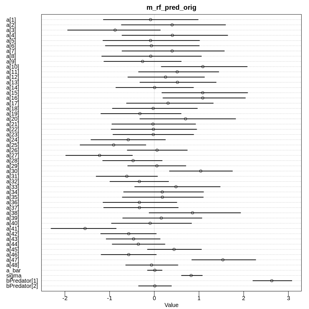
Raw data (preceding plot):
display(precis(m_rf_pred_orig, depth = 2), mimetypes="text/plain")
             mean         sd        5.5%       94.5%       n_eff     Rhat4
a[1]         -0.083782404 0.6683397 -1.1379711  0.97978035 3323.9971 1.0008964
a[2]          0.398279252 0.7445964 -0.7349006  1.59252908 3642.0880 1.0001770
a[3]         -0.876785015 0.6429685 -1.9377182  0.13439553 3238.1243 1.0000108
a[4]          0.404817552 0.7349930 -0.7216774  1.64137699 3915.5306 0.9999495
a[5]         -0.083832071 0.6807548 -1.1480278  1.01102351 4889.5287 0.9999990
a[6]         -0.064543360 0.6731676 -1.0929054  1.00604416 3752.6070 1.0003291
a[7]          0.399222684 0.7204982 -0.7208457  1.56588554 4585.0318 0.9997928
a[8]         -0.079077174 0.6930793 -1.1749677  1.05238137 3522.9661 0.9996251
a[9]         -0.261295201 0.5508050 -1.1253050  0.60100632 2317.3945 1.0012145
a[10]         1.086397196 0.6055322  0.1572343  2.07713264 2637.6138 1.0011137
a[11]         0.512536781 0.5545272 -0.3515829  1.44134523 3275.2223 0.9998713
a[12]         0.252246831 0.5413940 -0.5895404  1.12130573 3529.9706 1.0001809
a[13]         0.517606939 0.5409282 -0.3203855  1.38300840 3189.2797 0.9993446
a[14]         0.007966272 0.5452864 -0.8587002  0.87629608 3143.9566 1.0019361
a[15]         1.082976052 0.5940762  0.1704631  2.08731047 3125.6749 1.0013620
a[16]         1.083966838 0.5954497  0.1943514  2.03648723 2942.4873 1.0004327
a[17]         0.307882122 0.6211156 -0.6196864  1.31844413 3104.5980 1.0001957
a[18]        -0.024440129 0.5956933 -0.9353858  0.96297204 3050.9362 0.9999377
a[19]        -0.322044088 0.5594086 -1.1930236  0.59795057 2971.8151 1.0007469
a[20]         0.699363077 0.6770336 -0.3221011  1.81825238 3287.2801 0.9993965
a[21]        -0.029676017 0.5909633 -0.9473458  0.92240945 3799.2628 0.9997990
a[22]        -0.019969163 0.5951400 -0.9633570  0.94664701 2878.6961 1.0001915
a[23]        -0.022960338 0.5691990 -0.9237309  0.87953533 2941.1026 1.0001452
a[24]        -0.583188537 0.5318139 -1.4150223  0.24721705 2325.5757 1.0007251
a[25]        -0.908989744 0.4625179 -1.6597136 -0.18979408 2130.4492 1.0009958
a[26]         0.061814814 0.4106153 -0.6035636  0.73713222 1966.8725 1.0020998
a[27]        -1.223613568 0.4736511 -1.9801475 -0.49072337 2038.9436 1.0011452
a[28]        -0.474192041 0.4200759 -1.1532944  0.17521397 1902.3558 1.0021279
a[29]         0.058044075 0.4094488 -0.5928963  0.70524379 1658.2198 1.0019045
a[30]         1.039149281 0.4444185  0.3399477  1.74727794 2058.3658 1.0017041
a[31]        -0.614225356 0.4340739 -1.2999377  0.07114582 1831.4714 1.0015273
a[32]        -0.333502969 0.4134585 -0.9914475  0.31845742 1840.4414 1.0016380
a[33]         0.485086095 0.6032802 -0.4378054  1.47242921 3754.4555 0.9994368
a[34]         0.178130831 0.5629802 -0.6843041  1.10127152 3187.5376 0.9996313
a[35]         0.181149538 0.5619944 -0.7138831  1.09548978 3326.5974 1.0003590
a[36]        -0.333184898 0.5158115 -1.1461557  0.50254394 2765.2783 1.0010320
a[37]        -0.332305603 0.5208380 -1.1302133  0.53373571 3121.4519 1.0007885
a[38]         0.855190765 0.6652356 -0.1150859  1.92967540 2915.2388 0.9993069
a[39]         0.156371897 0.5568014 -0.7051821  1.06413438 3188.0402 0.9997562
a[40]        -0.093256217 0.5582221 -0.9565911  0.83181412 3187.7484 0.9997897
a[41]        -1.548553783 0.4514218 -2.3086019 -0.85330131 1741.3463 1.0012752
a[42]        -0.571494431 0.3900349 -1.1973287  0.04365076 1566.9078 1.0027316
a[43]        -0.463349086 0.3774608 -1.0749266  0.12959027 1653.0438 1.0024732
a[44]        -0.356041803 0.3652804 -0.9397087  0.23733724 1599.1564 1.0015854
a[45]         0.442376602 0.3774499 -0.1522825  1.05360378 1513.6236 1.0036103
a[46]        -0.571809119 0.3910414 -1.1878248  0.04423093 1870.2468 1.0012470
a[47]         1.534476766 0.4529039  0.8397431  2.26774186 1952.2301 1.0012205
a[48]        -0.062245170 0.3646090 -0.6385918  0.52738673 1440.0891 1.0015357
a_bar         0.012774764 0.1019977 -0.1517788  0.17333191 1165.2828 1.0022643
sigma         0.823758392 0.1463212  0.6090406  1.07356604 1304.0068 1.0012874
bPredator[1]  2.627815365 0.2733517  2.2066927  3.07630480 1194.8925 1.0016891
bPredator[2]  0.012354452 0.2266011 -0.3510555  0.38234517  701.2262 1.0064329
As explained above, this model struggles to sample. We’ve managed to avoid the warnings and achieve decent mixing by tightening a prior:
iplot(function() {
  traceplot(m_rf_pred_orig, pars=c("a[41]", "a[30]", "a_bar", "sigma", "bPredator[1]", "bPredator[2]"))
}, ar=2)
iplot(function() {
  trankplot(m_rf_pred_orig, pars=c("a[41]", "a[30]", "a_bar", "sigma", "bPredator[1]", "bPredator[2]"))
}, ar=2)
[1] 2000
[1] 1
[1] 2000
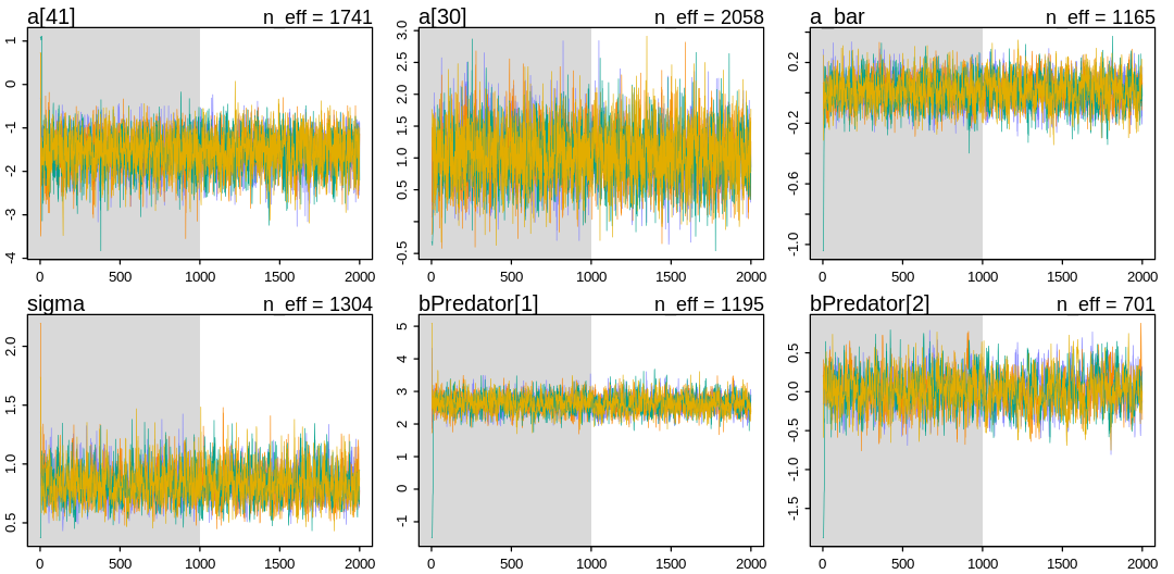
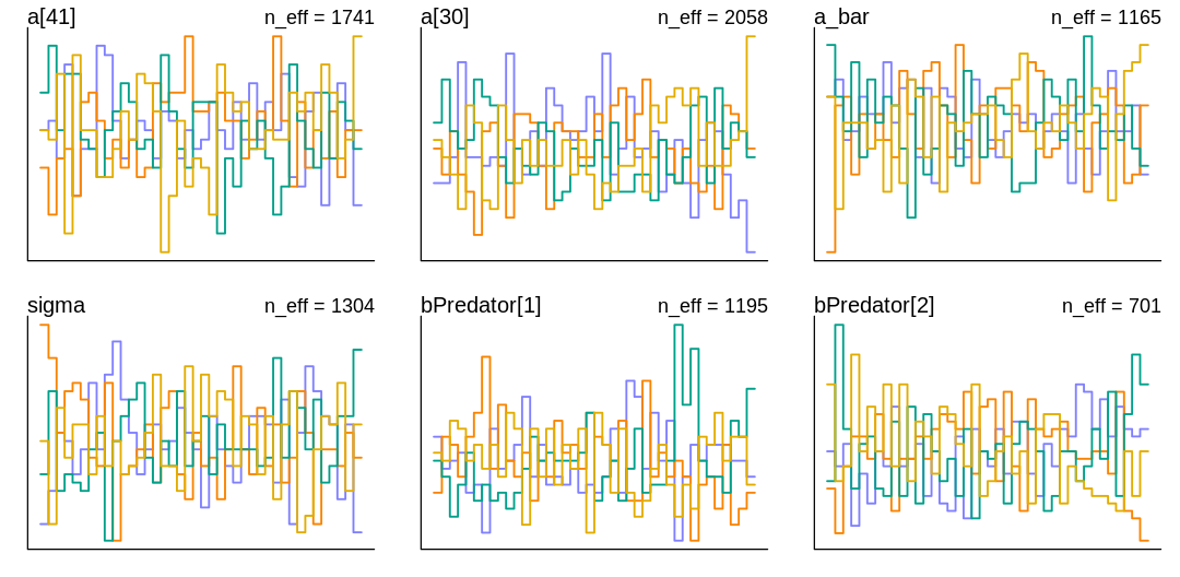
Why are we struggling to sample? To debug this, let’s go back to the chapter on debugging MCMC, in particular section 9.5.4. on non-identifiable parameters. If non-identifiable parameters are a cause of this symptom, what could we check for? Going even further back, to the end of section 6.1, the author suggests checking whether the posterior has changed relative to the prior. This is a good question to ask regularly; which parameters are unchanged relative to their prior? The obvious parameter is \(\bar{\alpha}\), which we already had to tweak. Let’s change the \(\bar{\alpha}\) prior again and see if it remains unchanged in the posterior:
m_rf_pred_shift <- ulam(
alist(
S ~ dbinom(N, p),
logit(p) <- a[tank] + bPredator[Predator],
a[tank] ~ dnorm(a_bar, sigma),
a_bar ~ dnorm(1.0, 0.1),
sigma ~ dexp(1),
bPredator[Predator] ~ dnorm(0, 1.5)
),
data = rf_dat, chains = 4, cores = 4, log_lik = TRUE, iter=2000
)
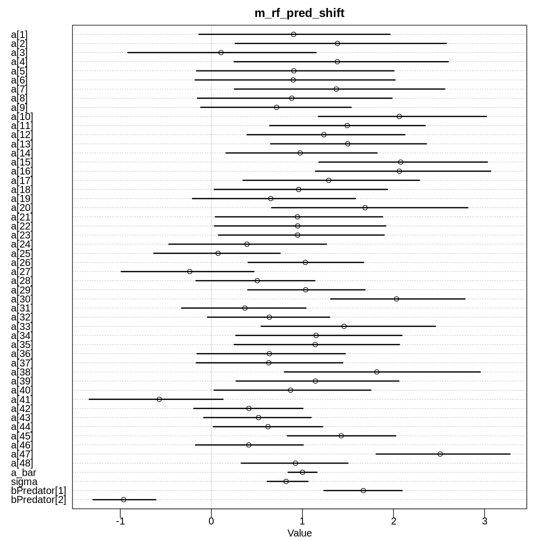
iplot(function() {
plot(precis(m_rf_pred_shift, depth=2), main='m_rf_pred_shift')
}, ar=1.0)
display_markdown("Raw data (preceding plot):")
display(precis(m_rf_pred_shift, depth = 2), mimetypes="text/plain")
Raw data (preceding plot):
             mean        sd         5.5%        94.5%      n_eff    Rhat4
a[1]          0.90354934 0.66198969 -0.13655045  1.9619029 4526.568 0.9995628
a[2]          1.38517848 0.73423364  0.26201324  2.5802182 4260.092 0.9997841
a[3]          0.10617791 0.65071668 -0.91620007  1.1496178 3653.841 1.0000794
a[4]          1.38328797 0.74142678  0.25096354  2.6013758 5064.727 0.9997997
a[5]          0.90552891 0.68725927 -0.16166813  2.0048297 6019.251 1.0004262
a[6]          0.89916921 0.68499725 -0.17918822  2.0171110 5219.442 0.9992895
a[7]          1.37223724 0.72998356  0.25312546  2.5626930 5598.259 0.9999840
a[8]          0.88311204 0.67620720 -0.15242976  1.9829023 5869.098 0.9991931
a[9]          0.71658141 0.51915095 -0.11673847  1.5353391 3156.780 1.0005604
a[10]         2.06411981 0.58258325  1.17676038  3.0206559 3985.056 1.0009753
a[11]         1.49176899 0.53598014  0.64111907  2.3479030 3860.228 1.0007428
a[12]         1.23569242 0.54458999  0.39207654  2.1249996 4257.877 1.0000510
a[13]         1.49786037 0.54380140  0.65004384  2.3615432 3837.861 1.0007850
a[14]         0.97498826 0.52162856  0.16155849  1.8195644 4187.411 1.0009462
a[15]         2.07883259 0.58609373  1.18209043  3.0301910 3005.062 1.0010137
a[16]         2.06413508 0.60510633  1.14390562  3.0677095 3854.658 1.0003025
a[17]         1.28879135 0.60933868  0.34805562  2.2850683 4338.382 0.9997227
a[18]         0.95959270 0.59298147  0.03233329  1.9342754 3886.468 1.0006232
a[19]         0.65196025 0.56212262 -0.20825662  1.5824422 4467.414 1.0000914
a[20]         1.68802102 0.67969301  0.66224142  2.8161560 3926.867 0.9997357
a[21]         0.94481301 0.57882890  0.04338898  1.8805384 4133.822 1.0015372
a[22]         0.94824457 0.59261456  0.03366506  1.9151639 4457.116 1.0003827
a[23]         0.94747270 0.56640838  0.07892487  1.8979849 4321.443 0.9998683
a[24]         0.39121062 0.53693899 -0.46628583  1.2633557 3282.330 1.0002785
a[25]         0.07376416 0.43981842 -0.63209917  0.7555797 2953.857 1.0010385
a[26]         1.03217452 0.40056580  0.40417642  1.6708940 2797.633 1.0022217
a[27]        -0.23707556 0.45841205 -0.98828970  0.4673189 3379.808 1.0007854
a[28]         0.50397668 0.40652291 -0.16836097  1.1363084 2733.469 1.0015429
a[29]         1.03586793 0.40703719  0.39959399  1.6865350 2708.253 1.0013806
a[30]         2.03313906 0.46170159  1.31050949  2.7850015 3033.605 1.0016206
a[31]         0.36904558 0.42537966 -0.32610087  1.0386976 2825.314 1.0014505
a[32]         0.63721349 0.41672026 -0.04216555  1.2996735 2640.202 1.0010433
a[33]         1.45749004 0.60246693  0.54642125  2.4595709 4119.071 0.9999246
a[34]         1.15012537 0.57404369  0.26897102  2.0920474 3981.452 1.0000701
a[35]         1.14070538 0.56727704  0.25169324  2.0648949 4178.897 0.9999761
a[36]         0.63721528 0.51019866 -0.15752427  1.4705572 3984.594 0.9998599
a[37]         0.63091757 0.51083414 -0.16554542  1.4432695 3975.426 0.9999726
a[38]         1.81656274 0.67220037  0.80206863  2.9524795 3559.289 0.9998314
a[39]         1.14190427 0.56659248  0.27273029  2.0590774 4035.939 1.0011109
a[40]         0.86922519 0.53211905  0.03078459  1.7516074 3828.537 1.0011976
a[41]        -0.57181635 0.45691531 -1.34014581  0.1283455 2393.828 1.0026273
a[42]         0.41222499 0.37976534 -0.19219483  1.0054733 2438.267 1.0023712
a[43]         0.51833068 0.37365220 -0.08345086  1.0958735 2570.765 1.0022313
a[44]         0.62228218 0.37804015  0.02154203  1.2223563 2481.839 1.0031281
a[45]         1.42563104 0.37187226  0.83409608  2.0245093 2401.124 1.0036513
a[46]         0.41104777 0.37012805 -0.17410541  1.0088594 2435.671 1.0023990
a[47]         2.51258631 0.45926259  1.81083124  3.2787478 2986.977 1.0013202
a[48]         0.92359732 0.36955612  0.32979850  1.4998346 2433.127 1.0034498
a_bar         1.00170337 0.09957427  0.84357080  1.1593070 1828.906 1.0022443
sigma         0.82049833 0.14199551  0.61383831  1.0609372 1247.405 1.0017245
bPredator[1]  1.66868730 0.26510181  1.23639294  2.0954120 1750.466 1.0021408
bPredator[2] -0.96206439 0.21494537 -1.30024438 -0.6094100 1007.932 1.0099470
The \(\bar{\alpha}\) prior remains unchanged even after being shifted. Notice that the predator
parameters are the ones that have responded (and unsuprisingly, all the a parameters). Previously
the model had inferred a ‘lack of predator’ drastically helps survival and a predator has no effect
on survival (treating a predator as the baseline). Now it has inferred a predator hurts chances of
survival, and the lack of a predator doesn’t help as much. That is, all these parameters only make
sense relative to each other.
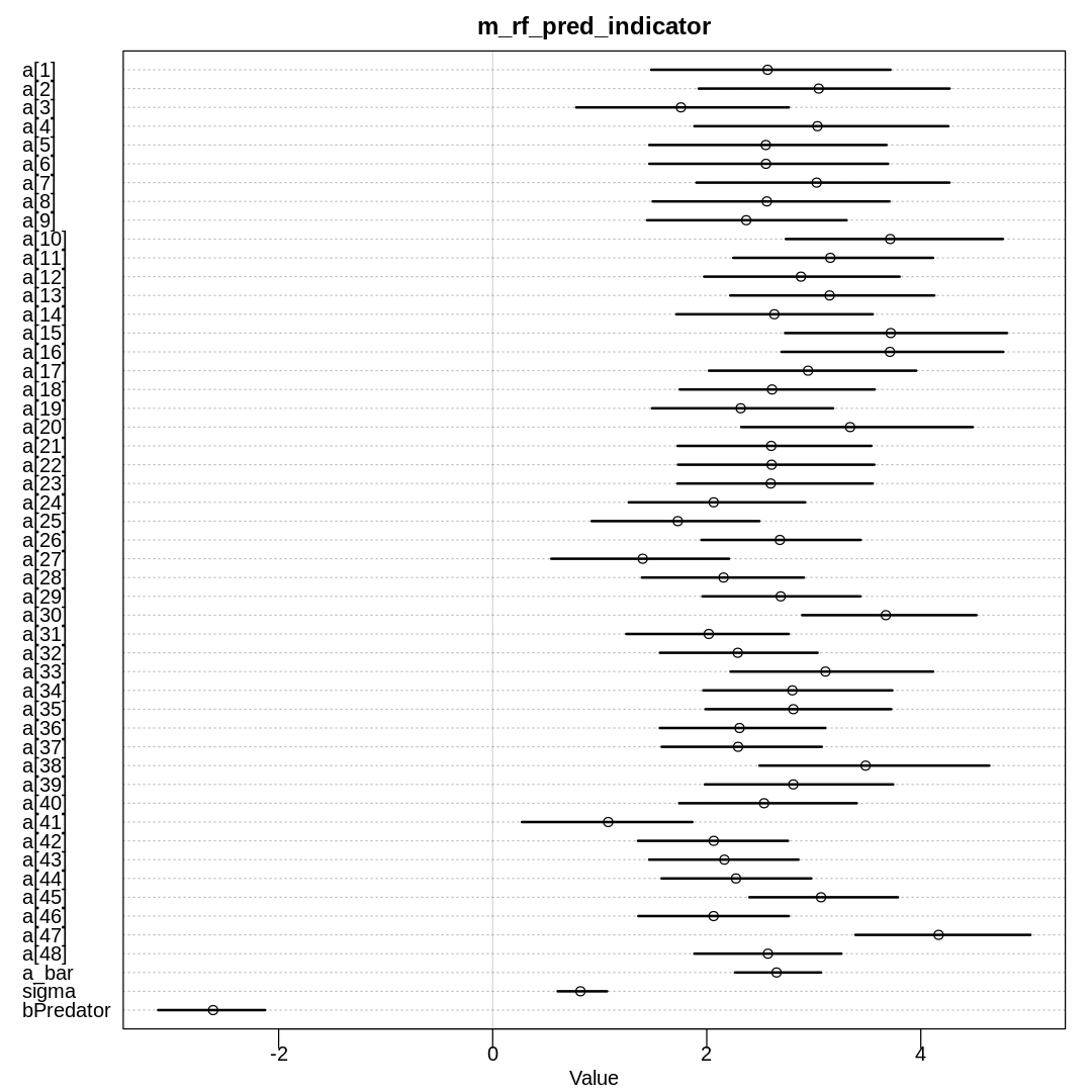
To avoid this mess we could use an indicator variable:
rf_dat <- list(
  S = rf_df$surv,
  N = rf_df$density,
  tank = rf_df$tank,
  Predator = ifelse(rf_df$Predator == 1, 0, 1)
)
m_rf_pred_indicator <- ulam(
  alist(
    S ~ dbinom(N, p),
    logit(p) <- a[tank] + bPredator * Predator,
    a[tank] ~ dnorm(a_bar, sigma),
    a_bar ~ dnorm(0, 2),
    sigma ~ dexp(1),
    bPredator ~ dnorm(0, 3)
  ),
  data = rf_dat, chains = 4, cores = 4, log_lik = TRUE, iter=4000
)

iplot(function() {
  plot(precis(m_rf_pred_indicator, depth=2), main='m_rf_pred_indicator')
}, ar=1.0)
display_markdown("Raw data (preceding plot):")
display(precis(m_rf_pred_indicator, depth = 2), mimetypes="text/plain")
Raw data (preceding plot):
          mean      sd        5.5%       94.5%     n_eff     Rhat4
a[1]       2.568625 0.7065333  1.4816095  3.716175 6496.2085 0.9997432
a[2]       3.046444 0.7392067  1.9249957  4.268914 4516.7295 1.0004573
a[3]       1.758601 0.6203789  0.7808663  2.767092 6149.3928 1.0002029
a[4]       3.034229 0.7531877  1.8839203  4.258121 4347.1198 1.0018325
a[5]       2.551850 0.6936042  1.4626645  3.679335 6506.9940 1.0000737
a[6]       2.553259 0.6972757  1.4635124  3.694513 7015.0622 1.0001421
a[7]       3.026929 0.7466069  1.9031680  4.267938 4751.9281 1.0005892
a[8]       2.561611 0.6926446  1.4948391  3.706838 5583.3152 1.0002331
a[9]       2.369040 0.5851668  1.4428870  3.306691 2802.2003 1.0006961
a[10]      3.714273 0.6335333  2.7387493  4.766806 2334.7544 1.0023544
a[11]      3.154776 0.5844844  2.2479629  4.115457 2380.0534 1.0014366
a[12]      2.880131 0.5721959  1.9755497  3.801759 2238.5121 1.0013077
a[13]      3.148154 0.5980840  2.2193946  4.126265 2342.8852 1.0016999
a[14]      2.631319 0.5694207  1.7160108  3.551355 2640.9382 1.0009717
a[15]      3.719320 0.6477859  2.7313733  4.804901 2295.9695 1.0013662
a[16]      3.712006 0.6444796  2.6983685  4.770902 2346.2489 1.0021495
a[17]      2.946438 0.6136488  2.0207754  3.957456 5035.0383 1.0005138
a[18]      2.610234 0.5708098  1.7466380  3.569257 6756.9365 1.0002097
a[19]      2.317044 0.5314623  1.4882151  3.180487 7555.4190 0.9999664
a[20]      3.339561 0.6788353  2.3222543  4.485846 5256.2067 1.0009351
a[21]      2.602672 0.5718423  1.7278342  3.538198 6630.7911 1.0000968
a[22]      2.605939 0.5705146  1.7314345  3.565800 6545.7650 1.0007736
a[23]      2.597704 0.5766954  1.7253049  3.551119 7171.8148 1.0001575
a[24]      2.064583 0.5173978  1.2714450  2.919533 7740.8052 0.9997146
a[25]      1.729316 0.4857999  0.9244728  2.491349 2044.2494 1.0022238
a[26]      2.683398 0.4679732  1.9503700  3.438943 1628.3831 1.0024543
a[27]      1.401694 0.5210254  0.5472158  2.208363 2051.3324 1.0032900
a[28]      2.156896 0.4691461  1.3943558  2.907548 1719.4547 1.0028071
a[29]      2.691007 0.4644481  1.9599637  3.435978 1665.4532 1.0019375
a[30]      3.673332 0.5154829  2.8916634  4.519748 1802.2092 1.0025643
a[31]      2.019034 0.4787989  1.2478532  2.765545 1784.2887 1.0021748
a[32]      2.289986 0.4638584  1.5624287  3.035747 1729.3579 1.0025040
a[33]      3.109471 0.5937000  2.2220242  4.115902 5782.7619 1.0005644
a[34]      2.800379 0.5505278  1.9670470  3.733864 6023.8347 0.9999593
a[35]      2.808822 0.5452622  1.9871573  3.723625 6092.2660 1.0005852
a[36]      2.306421 0.4838041  1.5615779  3.107488 7798.0167 0.9997884
a[37]      2.292929 0.4703855  1.5786414  3.075027 7134.5222 0.9999103
a[38]      3.484213 0.6771272  2.4923145  4.640025 3821.6583 1.0007627
a[39]      2.808635 0.5496937  1.9821605  3.741781 5290.3477 1.0005590
a[40]      2.535672 0.5149445  1.7420615  3.401859 6864.7004 1.0000298
a[41]      1.078934 0.5008621  0.2734995  1.865218 1965.0865 1.0018026
a[42]      2.065166 0.4397487  1.3579172  2.759018 1599.1369 1.0034113
a[43]      2.164809 0.4343670  1.4617999  2.856596 1411.1120 1.0025431
a[44]      2.273207 0.4387038  1.5781677  2.976636 1504.2018 1.0032525
a[45]      3.067862 0.4393549  2.3986873  3.786635 1509.9252 1.0037525
a[46]      2.064008 0.4370157  1.3606280  2.766340 1538.0953 1.0024969
a[47]      4.166467 0.5093548  3.3893331  5.024167 1738.8537 1.0024843
a[48]      2.571429 0.4338275  1.8835926  3.258263 1470.9813 1.0027349
a_bar      2.652263 0.2498896  2.2631389  3.068309  959.0550 1.0043707
sigma      0.820045 0.1462400  0.6071751  1.068717 1829.3086 1.0062332
bPredator -2.612418 0.3141985 -3.1260480 -2.126797  807.6546 1.0049977
Notice in the last model we’ve been able to widen the \(\bar{\alpha}\) prior and actually learn it from the data, that is, the prior changes in the posterior.
Still, an indicator variable isn’t ideal for at least one of the reasons given in section
5.3.1.: We aren’t more uncertain about the predator than the non-predator situation. The
indicator variable approach also makes it harder to read the a parameters relative to a_bar
since they aren’t centered at zero, and makes it harder to set an a_bar prior.
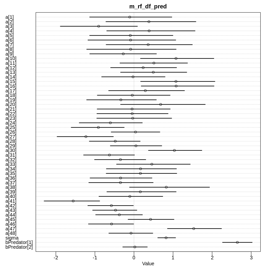
Instead let’s simply fix the a_bar prior’s expected value to zero as suggested in section
13.3.1:
rf_dat <- list(
  S = rf_df$surv,
  N = rf_df$density,
  tank = rf_df$tank,
  Predator = rf_df$Predator
)
m_rf_df_pred <- ulam(
  alist(
    S ~ dbinom(N, p),
    logit(p) <- a[tank] + bPredator[Predator],
    a[tank] ~ dnorm(0, sigma),
    sigma ~ dexp(1),
    bPredator[Predator] ~ dnorm(0, 1.5)
  ),
  data = rf_dat, chains = 4, cores = 4, log_lik = TRUE, iter=2000
)

iplot(function() {
  plot(precis(m_rf_df_pred, depth=2), main='m_rf_df_pred')
}, ar=1.0)
display_markdown("Raw data (preceding plot):")
display(precis(m_rf_df_pred, depth = 2), mimetypes="text/plain")
Raw data (preceding plot):
             mean        sd        5.5%       94.5%        n_eff     Rhat4
a[1]         -0.10926981 0.6678668 -1.1341574  0.968325113 6037.9640 0.9992977
a[2]          0.38245995 0.7232491 -0.7172980  1.583416429 5437.6276 0.9996457
a[3]         -0.90412695 0.6149605 -1.8853951  0.088430816 4426.5886 1.0003691
a[4]          0.38714333 0.7128869 -0.6966951  1.561855221 5808.5749 0.9997851
a[5]         -0.09492809 0.6766400 -1.1339914  0.996167302 5715.1859 0.9998989
a[6]         -0.08705118 0.6978017 -1.1780400  1.068730983 5655.9482 0.9997518
a[7]          0.36247985 0.6962178 -0.7126050  1.492395106 5067.3607 0.9998035
a[8]         -0.08554457 0.7030574 -1.2097559  1.077677940 5664.5541 0.9997368
a[9]         -0.27451498 0.5331677 -1.1310613  0.573933672 5485.9456 0.9996896
a[10]         1.07551160 0.5811640  0.1671313  2.044355615 4050.3845 1.0005275
a[11]         0.50905187 0.5371928 -0.3587378  1.368927180 5405.6542 1.0007624
a[12]         0.23397476 0.5316976 -0.5970856  1.089460567 4558.7970 0.9994633
a[13]         0.49392453 0.5308030 -0.3424429  1.350318285 4334.6663 1.0001892
a[14]        -0.02505129 0.5066164 -0.8272768  0.794122665 4431.1264 0.9995243
a[15]         1.07398074 0.6000142  0.1705671  2.070441147 3868.6025 0.9997723
a[16]         1.07861023 0.5863346  0.1852344  2.047903138 4364.7572 1.0014520
a[17]         0.29038749 0.6172948 -0.6485867  1.292898193 4837.2077 0.9998733
a[18]        -0.04417978 0.5806326 -0.9378659  0.923214650 5530.0816 0.9995366
a[19]        -0.33578511 0.5593470 -1.2116102  0.571323253 4126.0053 0.9998100
a[20]         0.68268797 0.6707529 -0.3430670  1.823845786 3927.8204 0.9996274
a[21]        -0.04966443 0.5829018 -0.9418029  0.925916104 4807.4597 0.9994333
a[22]        -0.04713234 0.5727702 -0.9484377  0.871924092 5115.6598 1.0001776
a[23]        -0.03238183 0.5908589 -0.9515834  0.963759145 5315.6278 0.9996640
a[24]        -0.60452921 0.5079522 -1.4008092  0.213217496 3965.6805 1.0005859
a[25]        -0.91182091 0.4309811 -1.6066943 -0.251241592 2518.3275 0.9992573
a[26]         0.03967339 0.3908975 -0.5834925  0.661842201 3272.4776 0.9999952
a[27]        -1.23062376 0.4498942 -1.9685776 -0.528943190 3052.8489 0.9997460
a[28]        -0.47992372 0.4073113 -1.1429065  0.157318608 3348.1390 0.9992844
a[29]         0.05018232 0.4074978 -0.6053623  0.710411241 2852.7053 1.0001879
a[30]         1.03454491 0.4248314  0.3705556  1.736136521 3470.5899 1.0002877
a[31]        -0.62844024 0.4089734 -1.2893593  0.011342839 3283.5912 0.9993627
a[32]        -0.34653369 0.4057128 -1.0088273  0.300833860 3433.6667 1.0004925
a[33]         0.45691465 0.5980984 -0.4458332  1.438866196 4038.9119 0.9998011
a[34]         0.16794070 0.5680171 -0.7063017  1.086086380 5106.1305 0.9993683
a[35]         0.16426638 0.5693969 -0.7111172  1.094543476 5033.9613 0.9992415
a[36]        -0.34204405 0.5024997 -1.1238248  0.459519205 4355.8346 0.9995794
a[37]        -0.34623090 0.5131147 -1.1560555  0.489964950 4768.8475 0.9993922
a[38]         0.82652012 0.6509020 -0.1139278  1.932964703 4134.6720 0.9998822
a[39]         0.16178476 0.5465724 -0.6924937  1.077661509 5135.6054 0.9998679
a[40]        -0.10579519 0.5122213 -0.8967349  0.735646613 4353.2567 1.0003343
a[41]        -1.55658794 0.4424122 -2.2995276 -0.879164833 2340.1845 1.0005009
a[42]        -0.57821358 0.3632792 -1.1809594 -0.017454635 2083.4559 0.9998722
a[43]        -0.47175809 0.3587480 -1.0579949  0.072774178 2493.3902 0.9995887
a[44]        -0.37516133 0.3783229 -0.9804668  0.215681914 2507.9463 1.0001557
a[45]         0.42476541 0.3647048 -0.1499028  1.023005732 2899.3842 1.0000727
a[46]        -0.57388435 0.3561543 -1.1648901 -0.009753087 2412.6051 0.9995497
a[47]         1.52936220 0.4338527  0.8577885  2.240218249 3220.1808 1.0010236
a[48]        -0.07552293 0.3535812 -0.6433861  0.480496241 2578.5205 0.9993191
sigma         0.82078371 0.1438559  0.6098134  1.064688346 1202.6301 1.0053265
bPredator[1]  2.64617315 0.2388067  2.2661468  3.024526582 1949.0686 1.0006127
bPredator[2]  0.02240382 0.1974405 -0.2865963  0.340611810  973.6414 1.0004159
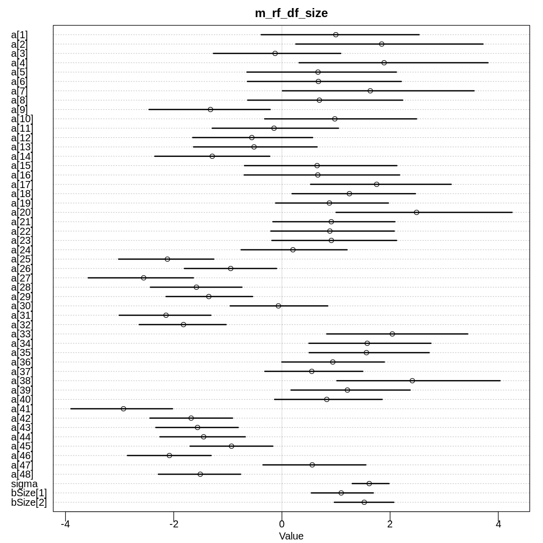
Let’s fit a similar model with only the size predictor:
rf_dat <- list(
  S = rf_df$surv,
  N = rf_df$density,
  tank = rf_df$tank,
  Size = rf_df$Size
)
m_rf_df_size <- ulam(
  alist(
    S ~ dbinom(N, p),
    logit(p) <- a[tank] + bSize[Size],
    a[tank] ~ dnorm(0, sigma),
    sigma ~ dexp(1),
    bSize[Size] ~ dnorm(0, 1.5)
  ),
  data = rf_dat, chains = 4, cores = 4, log_lik = TRUE, iter=2000
)

iplot(function() {
  plot(precis(m_rf_df_size, depth=2), main='m_rf_df_size')
}, ar=1.0)
display_markdown("Raw data (preceding plot):")
display(precis(m_rf_df_size, depth = 2), mimetypes="text/plain")
Raw data (preceding plot):
         mean        sd        5.5%         94.5%       n_eff     Rhat4
a[1]      0.99681519 0.9250799 -0.383461638  2.53653214 2338.6688 0.9993440
a[2]      1.84481606 1.0906502  0.256619448  3.71746959 3371.0629 1.0008074
a[3]     -0.12596782 0.7404463 -1.266160499  1.08735512 2151.3344 0.9995880
a[4]      1.88935339 1.1016899  0.317230320  3.80986954 2501.8406 1.0007815
a[5]      0.66709430 0.8868710 -0.646915875  2.11662993 2708.0392 1.0019113
a[6]      0.67465012 0.8938965 -0.637373357  2.20693727 3090.3661 1.0010968
a[7]      1.63347997 1.1099093  0.008668634  3.55292438 3179.5981 0.9999773
a[8]      0.69285128 0.9123927 -0.633128731  2.23307939 2320.5481 1.0008528
a[9]     -1.32075828 0.7067312 -2.456391922 -0.21675595 1877.3989 1.0002486
a[10]     0.97803274 0.8894598 -0.319442263  2.49011678 2650.1295 1.0004742
a[11]    -0.14591583 0.7395505 -1.288729076  1.04553223 2236.0944 0.9998969
a[12]    -0.55609702 0.7066487 -1.649493767  0.56874502 1962.8661 0.9995482
a[13]    -0.51526213 0.7168080 -1.633431317  0.65030477 1947.1120 1.0028663
a[14]    -1.28820210 0.6706377 -2.350219935 -0.22396521 1913.5004 1.0014835
a[15]     0.65048637 0.8857933 -0.692391470  2.12478241 2915.8382 1.0010854
a[16]     0.66368055 0.9140906 -0.698508882  2.17568918 3152.9088 1.0000158
a[17]     1.75157205 0.8206689  0.529602676  3.12943856 2651.4071 1.0001332
a[18]     1.24771340 0.7136876  0.186456188  2.46904542 1826.2568 0.9997428
a[19]     0.87778537 0.6547721 -0.116144812  1.96860598 1728.8694 1.0001824
a[20]     2.48949120 1.0110945  1.001199629  4.25503846 2155.5069 1.0002862
a[21]     0.91280229 0.7228677 -0.166828939  2.08877253 1771.2765 1.0017576
a[22]     0.88636155 0.7117838 -0.205452441  2.07772524 2365.6470 1.0019725
a[23]     0.91358999 0.7195110 -0.186363038  2.12019380 2505.7000 1.0006983
a[24]     0.20379570 0.6148468 -0.754644066  1.20448002 1669.3116 1.0037305
a[25]    -2.11689325 0.5539888 -3.019222433 -1.25882837 1434.1310 1.0004228
a[26]    -0.94714474 0.5313799 -1.803789604 -0.09803483 1224.2542 1.0000523
a[27]    -2.55589638 0.6043437 -3.581281601 -1.63595112 1427.0654 1.0016014
a[28]    -1.58048755 0.5358551 -2.430972220 -0.73880512 1172.9866 0.9999241
a[29]    -1.35128124 0.5059502 -2.142495644 -0.54040781 1346.0315 1.0036057
a[30]    -0.06489132 0.5693118 -0.956259443  0.84820454 1594.7748 1.0036467
a[31]    -2.14226335 0.5286497 -3.008090728 -1.31336512 1351.3011 1.0048746
a[32]    -1.81960353 0.5036942 -2.638933470 -1.03182329 1369.6956 1.0035545
a[33]     2.04107295 0.8158143  0.828710202  3.43507386 1796.0666 1.0007612
a[34]     1.57751184 0.7087987  0.498944547  2.75549887 1836.2079 0.9997244
a[35]     1.56225901 0.6873602  0.503008718  2.72298088 1654.3252 1.0010555
a[36]     0.94052548 0.5988971 -0.002387076  1.89449712 1427.5108 1.0000394
a[37]     0.55169564 0.5737066 -0.316323393  1.49562078 1456.2497 1.0024331
a[38]     2.41067355 0.9725551  1.015315398  4.03270783 2738.9698 1.0007341
a[39]     1.21065821 0.6990039  0.168437603  2.37037485 2375.4872 1.0013355
a[40]     0.82921161 0.6208004 -0.136016908  1.85353169 1840.3297 1.0028235
a[41]    -2.92896461 0.5843685 -3.901165309 -2.02204732 1433.7926 1.0001028
a[42]    -1.67802853 0.4854459 -2.439864529 -0.91229357 1056.4477 1.0007244
a[43]    -1.55998959 0.4822083 -2.331878922 -0.80779980  988.4055 1.0012142
a[44]    -1.44712397 0.4876699 -2.254768648 -0.67772817 1081.0996 1.0007491
a[45]    -0.93148328 0.4814104 -1.697659746 -0.16725127 1080.5924 1.0045373
a[46]    -2.07986789 0.4781940 -2.855888562 -1.30903556 1239.7636 1.0039279
a[47]     0.56055844 0.5962120 -0.349575631  1.55259310 1766.9219 1.0027201
a[48]    -1.50919169 0.4727175 -2.284075803 -0.76360834 1231.1176 1.0041877
sigma     1.61423267 0.2167541  1.299284035  1.98046591 2013.0327 1.0005588
bSize[1]  1.09626817 0.3593848  0.543652132  1.68996240  644.6992 1.0007952
bSize[2]  1.52185411 0.3402183  0.969055130  2.06942872  711.6491 1.0096700
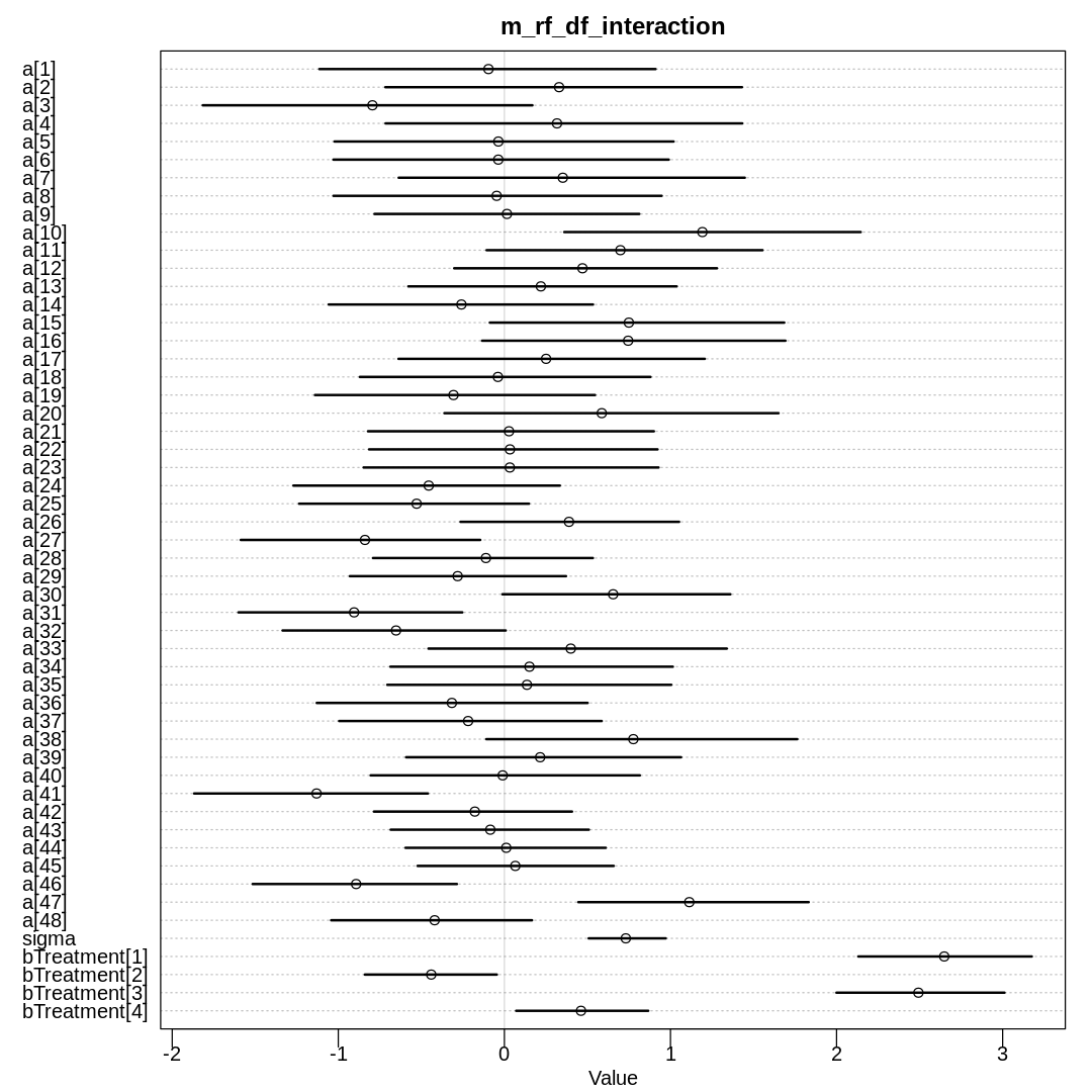
Finally, lets model an interaction term. We’ve already added a ‘treatment’ index variable in preprocessing; see the data.frame near the start of this question.
rf_dat <- list(
  S = rf_df$surv,
  N = rf_df$density,
  tank = rf_df$tank,
  Treatment = rf_df$Treatment
)
m_rf_df_interaction <- ulam(
  alist(
    S ~ dbinom(N, p),
    logit(p) <- a[tank] + bTreatment[Treatment],
    a[tank] ~ dnorm(0, sigma),
    sigma ~ dexp(1),
    bTreatment[Treatment] ~ dnorm(0, 1.5)
  ),
  data = rf_dat, chains = 4, cores = 4, log_lik = TRUE, iter=2000
)

iplot(function() {
  plot(precis(m_rf_df_interaction, depth=2), main='m_rf_df_interaction')
}, ar=1.0)
display_markdown("Raw data (preceding plot):")
display(precis(m_rf_df_interaction, depth = 2), mimetypes="text/plain")
Raw data (preceding plot):
              mean        sd        5.5%        94.5%        n_eff    Rhat4
a[1]          -0.09577943 0.6267033 -1.11367532  0.909977164 5143.005 1.0007719
a[2]           0.32937745 0.6666951 -0.71629499  1.430401615 4567.441 0.9998441
a[3]          -0.79443631 0.6215156 -1.81581619  0.168699311 2976.359 0.9997780
a[4]           0.31684711 0.6624686 -0.71535948  1.432068943 4022.641 0.9997259
a[5]          -0.03627342 0.6268386 -1.02283906  1.018770230 4735.669 0.9996099
a[6]          -0.03674150 0.6348940 -1.02943757  0.989733158 4307.582 0.9996470
a[7]           0.35181370 0.6562340 -0.63623773  1.447407734 4558.268 1.0000299
a[8]          -0.04647555 0.6309091 -1.02917035  0.946866389 4134.329 0.9994656
a[9]           0.01536831 0.5000787 -0.78205408  0.812041588 4670.907 0.9995015
a[10]          1.19215902 0.5616020  0.36068617  2.145145015 2644.889 1.0004477
a[11]          0.69860943 0.5211471 -0.10694401  1.554137875 3494.254 0.9997648
a[12]          0.47016846 0.4929578 -0.30206100  1.279733362 3501.187 1.0001560
a[13]          0.21964163 0.5105650 -0.57824370  1.037172708 5033.794 1.0001793
a[14]         -0.25871092 0.5005928 -1.05757485  0.533512546 4076.583 0.9999903
a[15]          0.74946846 0.5612220 -0.08737410  1.684836342 3677.212 1.0004659
a[16]          0.74506582 0.5791291 -0.13406370  1.691922384 3767.438 0.9997133
a[17]          0.25101101 0.5742688 -0.63749945  1.206408241 4444.808 0.9995868
a[18]         -0.03890772 0.5427108 -0.87009914  0.879598757 4083.113 0.9995462
a[19]         -0.30640879 0.5242328 -1.14032337  0.545403272 3858.947 0.9994792
a[20]          0.58633708 0.6359119 -0.36086156  1.650452505 3816.377 0.9997111
a[21]          0.02777862 0.5358812 -0.82106937  0.900102835 4180.677 0.9997157
a[22]          0.03350398 0.5434988 -0.81427365  0.922278762 4463.592 1.0003012
a[23]          0.03268665 0.5463121 -0.84743321  0.928045896 4247.752 0.9998151
a[24]         -0.45556983 0.5062522 -1.27002390  0.333963820 4646.453 0.9996221
a[25]         -0.52834454 0.4368545 -1.23562709  0.147793291 3145.816 1.0002173
a[26]          0.38909402 0.4112371 -0.26396123  1.051841876 2956.467 1.0012036
a[27]         -0.83944227 0.4605587 -1.58721306 -0.145213912 2839.272 1.0001094
a[28]         -0.11124511 0.4067748 -0.79105363  0.532770771 2793.868 1.0012389
a[29]         -0.28139357 0.4016775 -0.93017893  0.370981895 2400.101 1.0007431
a[30]          0.65475297 0.4310860 -0.01195392  1.360445231 3021.429 1.0008335
a[31]         -0.90486633 0.4221398 -1.60081764 -0.253605028 2539.958 1.0009230
a[32]         -0.65228788 0.4158850 -1.33532431  0.008000418 2478.460 1.0012881
a[33]          0.39974166 0.5697229 -0.45712801  1.338927728 4693.496 0.9994861
a[34]          0.15096088 0.5361788 -0.68610362  1.014130485 4696.179 1.0000059
a[35]          0.13591497 0.5391028 -0.70472650  1.004612067 4458.872 0.9992013
a[36]         -0.31609573 0.5104419 -1.12969763  0.501306825 3276.943 1.0001300
a[37]         -0.21838802 0.4865336 -0.99477115  0.585942405 3814.917 1.0003465
a[38]          0.77644583 0.5945447 -0.10859117  1.763270260 3420.977 1.0003442
a[39]          0.21537604 0.5186425 -0.59158651  1.063760756 4164.077 1.0006626
a[40]         -0.01023445 0.5101771 -0.80499991  0.815480415 4006.309 0.9996398
a[41]         -1.13073829 0.4360626 -1.86773448 -0.460772871 2554.749 1.0010795
a[42]         -0.17779774 0.3785500 -0.78533913  0.407278264 2815.529 1.0012546
a[43]         -0.08475116 0.3702704 -0.68437932  0.508510725 2658.990 1.0015944
a[44]          0.01115516 0.3720450 -0.59496876  0.609996991 2594.928 1.0003085
a[45]          0.06577529 0.3719377 -0.52249992  0.658075119 2594.179 1.0003444
a[46]         -0.89262279 0.3880924 -1.51537072 -0.286113711 2159.221 1.0019371
a[47]          1.11322450 0.4370110  0.44549412  1.831845876 2636.593 1.0013490
a[48]         -0.42004752 0.3720838 -1.04267696  0.166230236 2394.195 1.0019273
sigma          0.73100956 0.1454545  0.50768595  0.971485925 1023.207 1.0036739
bTreatment[1]  2.64821704 0.3238602  2.13078698  3.175377341 2295.982 1.0003074
bTreatment[2] -0.44039782 0.2532552 -0.84011033 -0.045516758 1463.127 1.0022765
bTreatment[3]  2.49272498 0.3121271  1.99944824  3.010880805 2383.259 0.9998855
bTreatment[4]  0.46123019 0.2516495  0.07106990  0.865870231 1278.665 1.0047769
Let’s go back to the original question:
Instead of focusing on inferences about these two predictor variables, focus on the inferred variation across tanks. Explain why it changes as it does across models.
The inferred variation across tanks (\(\sigma\)) decreases in these models as we add more predictors.
We see the largest \(\sigma\) in m13.2 where we haven’t tried to explain variation with any
predictors. When we add the predator predictor in m_rf_df_pred we see sigma drop significantly
because there is a lot of predictive power in that variable (or at least more than size). The
model with an interaction term has the lowest inference for sigma because it indirectly has access
to all the predictors.
One question only exists in 13H4:
What do you infer about the causal inference of these predictor variables?
In the typical predator-prey relationship it’s more appropriate to use differential equations to model the relationship between the populations. Reading the original paper, though, it appears that the presence of predators, tadpole sizes, and initial density were manipulated. If that is the case then the causal diagram would be relatively simple: the predictors can only affect the outcome, not each other.
It’s tempting to read from the difference between bTreatment[1] and bTreatment[3] relative to
the difference between bTreatment[2] and bTreatment[4] that being large helps survival in the
absence of predators (to overcome the elements/nature) but in the presence of predators being large
makes a tadpole easier to catch (harder to hide) and more desirable to catch.
The support for the advantage of size in the absence of predators is limited, though, considering
the error bars on bTreatment[1] and bTreatment[3]. If we only accept the significant difference
in survivability from being smaller in the presence of predators, we would conclude being small
would primarily be an advantage in the larval/tadpole stage of the frog’s development without an
explanation for why some tadpoles hatch larger. Based on the original paper, the confounding
variable seems to be survivability at metamorphosis, which could influence the timing of hatching
and therefore the ideal tadpole size. Tadpoles that are smaller at metamorphosis may be less likely
to survive (or reproduce) than those that are larger.
That is, there are two influences on the ideal tadpole size, both survivability at life stages in nature:
MetaSurv -> TadpoleSize <- LarvSurv
The species (apparently) has to tradeoff size to survive both stages.
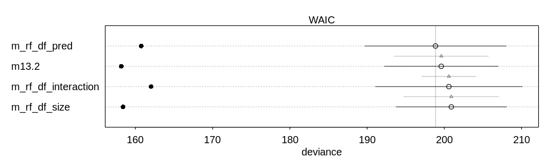
13M2. Compare the models you fit just above, using WAIC. Can you reconcile the differences in WAIC with the posterior distributions of the models?
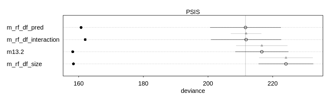
Answer. For comparison and to check on warnings, these results include PSIS deviances as well.
Notice the model with the predator predictor does well in both comparisons. This predictor
significantly improves predictive accuracy at the cost of only one parameter. Generally speaking the
model with only the size predictor does not do as well, because (alone) this is not an effective
predictor of whether the tadpole will survive to metamorphosis.
In general there are not large differences between these models, however, considering the error bars produced by both WAIC and PSIS.
iplot(function() {
  plot(compare(m13.2, m_rf_df_pred, m_rf_df_size, m_rf_df_interaction))
}, ar=3.5)
display_markdown("Raw data (preceding plot):")
display(compare(m13.2, m_rf_df_pred, m_rf_df_size, m_rf_df_interaction), mimetypes="text/plain")

p_comp = compare(m13.2, m_rf_df_pred, m_rf_df_size, m_rf_df_interaction, func=PSIS)
iplot(function() {
  plot(p_comp)
}, ar=3.5)
display_markdown("Raw data (preceding plot):")
display(p_comp, mimetypes="text/plain")
Raw data (preceding plot):
                    WAIC     SE       dWAIC     dSE      pWAIC    weight
m_rf_df_pred        198.8568 9.147986 0.0000000       NA 19.05042 0.4050145
m13.2               199.6016 7.359110 0.7447747 6.115536 20.71044 0.2790903
m_rf_df_interaction 200.5899 9.522778 1.7330538 3.522336 19.27701 0.1702718
m_rf_df_size        200.9026 7.157208 2.0457976 6.171391 21.24540 0.1456234
Some Pareto k values are very high (>1). Set pointwise=TRUE to inspect individual points.
Some Pareto k values are very high (>1). Set pointwise=TRUE to inspect individual points.
Some Pareto k values are very high (>1). Set pointwise=TRUE to inspect individual points.
Some Pareto k values are very high (>1). Set pointwise=TRUE to inspect individual points.
Raw data (preceding plot):
                    PSIS     SE        dPSIS      dSE      pPSIS
m_rf_df_pred        211.5875 10.925181  0.0000000       NA 25.41577
m_rf_df_interaction 211.7769 10.843066  0.1893256 4.710982 24.87049
m13.2               216.6323  8.185321  5.0447690 7.929426 29.22578
m_rf_df_size        224.0973  8.445160 12.5097871 8.285123 32.84273
                    weight
m_rf_df_pred        0.5020411436
m_rf_df_interaction 0.4566965917
m13.2               0.0402978284
m_rf_df_size        0.0009644363
13M3. Re-estimate the basic Reed frog varying intercept model, but now using a Cauchy distribution in place of the Gaussian distribution for the varying intercepts. That is, fit this model:
(You are likely to see many divergent transitions for this model. Can you figure out why? Can you fix them?) Compare the posterior means of the intercepts, \(\alpha_{tank}\), to the posterior means produced in the chapter, using the customary Gaussian prior. Can you explain the pattern of differences? Take note of any change in the mean \(\alpha\) as well.
Answer. First, let’s reproduce some of the plots from the chapter. Similar to the approach in
the R code 13.22 box and elsewhere, we’ll print the raw output of precis for a model before its
plots:
data(reedfrogs)
rf_df <- reedfrogs
rf_df$tank <- 1:nrow(rf_df)
rf_dat <- list(
S = rf_df$surv,
N = rf_df$density,
tank = rf_df$tank
)
## R code 13.3
m13.2 <- ulam(
alist(
S ~ dbinom(N, p),
logit(p) <- a[tank],
a[tank] ~ dnorm(a_bar, sigma),
a_bar ~ dnorm(0, 1.5),
sigma ~ dexp(1)
),
data = rf_dat, chains = 4, cores = 4, log_lik = TRUE
)
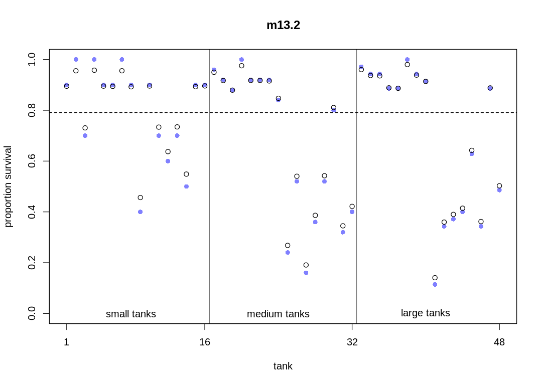
plot_means <- function(post, plot_main) {
# compute mean intercept for each tank
# also transform to probability with logistic
rf_df$propsurv.est <- logistic(apply(post$a, 2, mean))
iplot(function() {
# display raw proportions surviving in each tank
plot(rf_df$propsurv,
ylim = c(0, 1), pch = 16, xaxt = "n",
xlab = "tank", ylab = "proportion survival", col = rangi2,
main=plot_main
)
axis(1, at = c(1, 16, 32, 48), labels = c(1, 16, 32, 48))
# overlay posterior means
points(rf_df$propsurv.est)
# mark posterior mean probability across tanks
abline(h = mean(inv_logit(post$a_bar)), lty = 2)
# draw vertical dividers between tank densities
abline(v = 16.5, lwd = 0.5)
abline(v = 32.5, lwd = 0.5)
text(8, 0, "small tanks")
text(16 + 8, 0, "medium tanks")
text(32 + 8, 0, "large tanks")
})
}
display(precis(m13.2, depth = 2), mimetypes="text/plain")
iplot(function() {
plot(precis(m13.2, depth=2), main='m13.2')
}, ar=1.0)
post <- extract.samples(m13.2)
plot_means(post, "m13.2")
      mean        sd        5.5%        94.5%         n_eff    Rhat4
a[1]   2.14141939 0.9227311  0.80304567  3.7232490746 3019.959 0.9988686
a[2]   3.06845529 1.1245458  1.45798211  5.0515349796 3032.690 0.9987560
a[3]   0.99872572 0.6593702  0.03008953  2.0663935974 4248.298 0.9987840
a[4]   3.12183560 1.1671522  1.45394347  5.2163175434 2583.453 1.0011453
a[5]   2.14487025 0.8674482  0.87431847  3.6786839542 2980.456 0.9996371
a[6]   2.13494908 0.8810399  0.82115520  3.6273644969 4250.483 0.9988450
a[7]   3.07043122 1.0628488  1.50652736  4.9149981884 2999.425 0.9993862
a[8]   2.11639350 0.8624158  0.86311767  3.5654573096 3691.015 0.9988983
a[9]  -0.17451773 0.6160772 -1.17906263  0.7781815875 4412.903 0.9985298
a[10]  2.14924350 0.8666111  0.86749380  3.6574129203 3657.996 0.9989235
a[11]  1.01360166 0.6960467 -0.04851253  2.1632821028 4218.045 0.9991958
a[12]  0.56365385 0.6364008 -0.40873922  1.5739370873 6438.407 0.9985277
a[13]  1.01835187 0.6689844  0.01354333  2.1057665866 4706.569 0.9996362
a[14]  0.19562294 0.6150966 -0.79479926  1.1996435479 4475.824 0.9994110
a[15]  2.12001815 0.8747703  0.83979645  3.6501388962 3158.016 0.9988068
a[16]  2.15345623 0.8889400  0.84845843  3.6691164332 3210.056 0.9999396
a[17]  2.93672781 0.8223109  1.73731451  4.3327202679 2664.294 0.9989159
a[18]  2.40456148 0.6887045  1.36081786  3.5724183540 3587.124 0.9987023
a[19]  1.98598674 0.5506898  1.14984136  2.9194434039 4154.275 0.9987964
a[20]  3.68161659 1.0180129  2.24736057  5.4223735078 2915.105 0.9988011
a[21]  2.40890546 0.6823749  1.41394392  3.5318284276 4104.421 0.9984927
a[22]  2.40879997 0.6919729  1.37779325  3.6041313689 3338.300 1.0003087
a[23]  2.38303819 0.6507824  1.40724398  3.4821347055 3787.105 0.9985278
a[24]  1.71372196 0.5208176  0.91564841  2.5799636306 4313.543 0.9998662
a[25] -1.00432263 0.4289957 -1.66623476 -0.3494891073 5211.070 0.9986643
a[26]  0.16132993 0.4002201 -0.47590580  0.7989392568 4907.484 0.9995734
a[27] -1.44379137 0.5072702 -2.28628083 -0.6685400488 4580.331 0.9990651
a[28] -0.46235557 0.4185657 -1.13114708  0.2006028455 5922.888 0.9981964
a[29]  0.16917263 0.4062452 -0.48489757  0.8080211423 4654.534 0.9988287
a[30]  1.45504716 0.5071826  0.67726561  2.3257112135 4784.827 0.9983597
a[31] -0.64066006 0.3940076 -1.28024056 -0.0156096245 5253.508 0.9984616
a[32] -0.31596411 0.4092429 -0.96633689  0.3402954733 3428.362 0.9985635
a[33]  3.18504972 0.7807287  2.08075055  4.5536010019 2948.638 0.9989894
a[34]  2.69718467 0.6089541  1.81831617  3.7092264503 3951.260 0.9989309
a[35]  2.67554574 0.6095605  1.76148379  3.6546226616 3908.349 0.9985476
a[36]  2.07452480 0.5142351  1.30491029  2.9420774710 3776.388 0.9993834
a[37]  2.05810630 0.5205456  1.27821922  2.9200066620 3853.280 0.9986392
a[38]  3.89399516 0.9894540  2.51940551  5.5738973919 2593.062 0.9997222
a[39]  2.72601789 0.6652081  1.75377465  3.8073063458 4458.028 0.9983142
a[40]  2.35945817 0.5722368  1.52207351  3.2916018001 3695.220 0.9982091
a[41] -1.80837069 0.4875161 -2.61878771 -1.0617814169 4421.013 0.9987071
a[42] -0.57650848 0.3696980 -1.18852830  0.0004745021 4785.780 0.9983363
a[43] -0.44683424 0.3361611 -0.99731996  0.0726275019 3837.253 0.9993585
a[44] -0.34555342 0.3164648 -0.85716025  0.1429417871 3702.156 0.9996123
a[45]  0.58520174 0.3611214  0.02318340  1.1701626320 4340.697 0.9985885
a[46] -0.56655543 0.3487765 -1.12545837 -0.0397354141 3740.114 0.9984123
a[47]  2.07195447 0.5202763  1.28991954  2.9607066812 3060.582 1.0005639
a[48]  0.01069638 0.3393415 -0.52418876  0.5369077391 3866.338 0.9992965
a_bar  1.34866871 0.2556178  0.95208750  1.7612201878 2554.061 0.9987120
sigma  1.62246318 0.2121107  1.30549715  1.9833010376 1840.111 0.9993955
As promised, sampling from the model produces divergent transitions:
m_tank_cauchy_orig <- ulam(
  alist(
    S ~ dbinom(N, p),
    logit(p) <- a[tank],
    a[tank] ~ dcauchy(a_bar, sigma),
    a_bar ~ dnorm(0, 1),
    sigma ~ dexp(1)
  ),
  data = rf_dat, chains = 4, cores = 4, log_lik = TRUE
)
Warning message:
“There were 160 divergent transitions after warmup. See
https://mc-stan.org/misc/warnings.html#divergent-transitions-after-warmup
to find out why this is a problem and how to eliminate them.”
Warning message:
“Examine the pairs() plot to diagnose sampling problems
”
Warning message:
“Bulk Effective Samples Size (ESS) is too low, indicating posterior means and medians may be unreliable.
Running the chains for more iterations may help. See
https://mc-stan.org/misc/warnings.html#bulk-ess”
Warning message:
“Tail Effective Samples Size (ESS) is too low, indicating posterior variances and tail quantiles may be unreliable.
Running the chains for more iterations may help. See
https://mc-stan.org/misc/warnings.html#tail-ess”
Adjusting adapt_delta does little to reduce the number of divergent transitions:
m_tank_cauchy <- ulam(
  alist(
    S ~ dbinom(N, p),
    logit(p) <- a[tank],
    a[tank] ~ dcauchy(a_bar, sigma),
    a_bar ~ dnorm(0, 1),
    sigma ~ dexp(1)
  ),
  data = rf_dat, chains = 4, cores = 4, log_lik = TRUE, control=list(adapt_delta=0.99)
)
recompiling to avoid crashing R session
Warning message:
“There were 132 divergent transitions after warmup. See
https://mc-stan.org/misc/warnings.html#divergent-transitions-after-warmup
to find out why this is a problem and how to eliminate them.”
Warning message:
“Examine the pairs() plot to diagnose sampling problems
”
Warning message:
“Tail Effective Samples Size (ESS) is too low, indicating posterior variances and tail quantiles may be unreliable.
Running the chains for more iterations may help. See
https://mc-stan.org/misc/warnings.html#tail-ess”
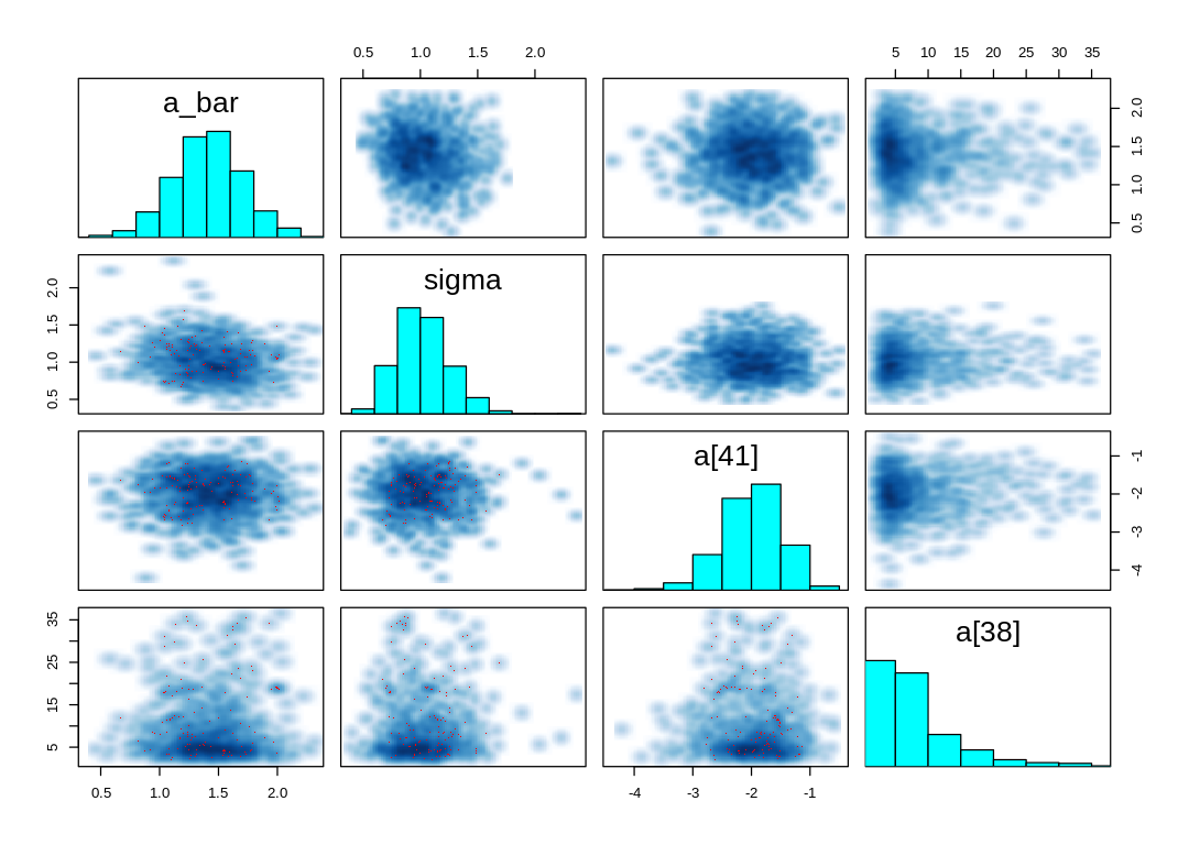
Let’s examine the pairs() plot suggested in the warning message (for only a few parameters):
sel_pars = c("a_bar", "sigma", "a[41]", "a[38]")
iplot(function() {
pairs(m_tank_cauchy@stanfit, pars=sel_pars)
})
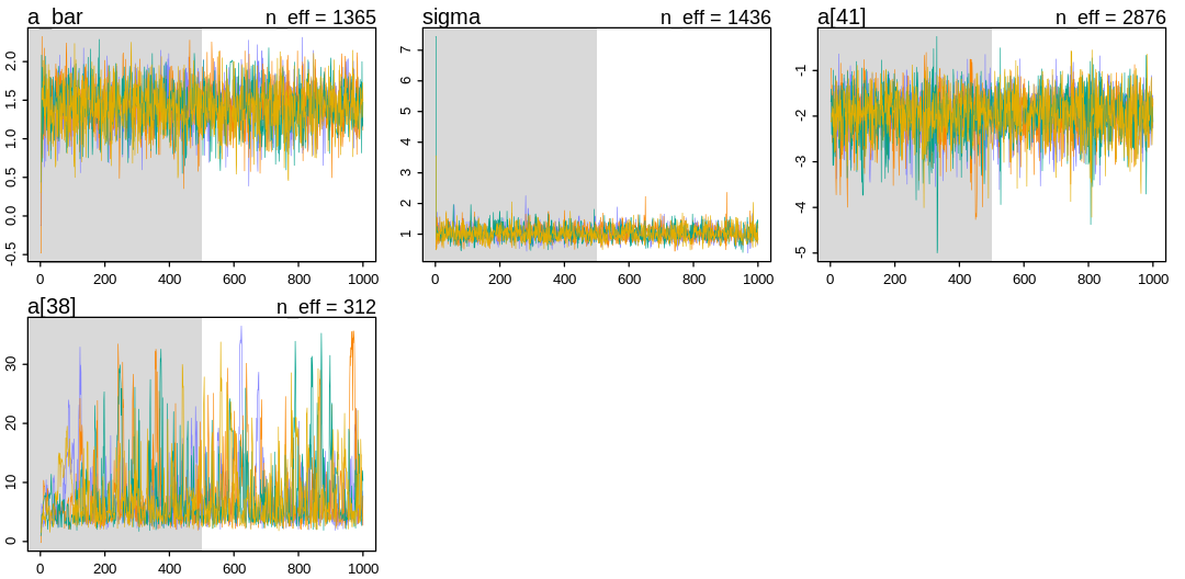
iplot(function() {
traceplot(m_tank_cauchy, pars=sel_pars)
}, ar=2)
[1] 1000
[1] 1
[1] 1000
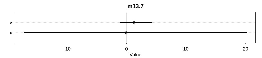
For comparison, these are the same plots for the Devil’s Funnel (i.e. Neal’s Funnel):
m13.7 <- ulam(
  alist(
    v ~ normal(0, 3),
    x ~ normal(0, exp(v))
  ),
  data = list(N = 1), chains = 4
)
display(precis(m13.7), mimetypes="text/plain")
iplot(function() {
  plot(precis(m13.7), main='m13.7')
}, ar=4.5)
SAMPLING FOR MODEL '3a5530af995ac1418f5e59b7607ceed3' NOW (CHAIN 1).
Chain 1:
Chain 1: Gradient evaluation took 7e-06 seconds
Chain 1: 1000 transitions using 10 leapfrog steps per transition would take 0.07 seconds.
Chain 1: Adjust your expectations accordingly!
Chain 1:
Chain 1:
Chain 1: Iteration:   1 / 1000 [  0%]  (Warmup)
Chain 1: Iteration: 100 / 1000 [ 10%]  (Warmup)
Chain 1: Iteration: 200 / 1000 [ 20%]  (Warmup)
Chain 1: Iteration: 300 / 1000 [ 30%]  (Warmup)
Chain 1: Iteration: 400 / 1000 [ 40%]  (Warmup)
Chain 1: Iteration: 500 / 1000 [ 50%]  (Warmup)
Chain 1: Iteration: 501 / 1000 [ 50%]  (Sampling)
Chain 1: Iteration: 600 / 1000 [ 60%]  (Sampling)
Chain 1: Iteration: 700 / 1000 [ 70%]  (Sampling)
Chain 1: Iteration: 800 / 1000 [ 80%]  (Sampling)
Chain 1: Iteration: 900 / 1000 [ 90%]  (Sampling)
Chain 1: Iteration: 1000 / 1000 [100%]  (Sampling)
Chain 1:
Chain 1:  Elapsed Time: 0.023276 seconds (Warm-up)
Chain 1:                0.013432 seconds (Sampling)
Chain 1:                0.036708 seconds (Total)
Chain 1:

SAMPLING FOR MODEL '3a5530af995ac1418f5e59b7607ceed3' NOW (CHAIN 2).
Chain 2:
Chain 2: Gradient evaluation took 3e-06 seconds
Chain 2: 1000 transitions using 10 leapfrog steps per transition would take 0.03 seconds.
Chain 2: Adjust your expectations accordingly!
Chain 2:
Chain 2:
Chain 2: Iteration:   1 / 1000 [  0%]  (Warmup)
Chain 2: Iteration: 100 / 1000 [ 10%]  (Warmup)
Chain 2: Iteration: 200 / 1000 [ 20%]  (Warmup)
Chain 2: Iteration: 300 / 1000 [ 30%]  (Warmup)
Chain 2: Iteration: 400 / 1000 [ 40%]  (Warmup)
Chain 2: Iteration: 500 / 1000 [ 50%]  (Warmup)
Chain 2: Iteration: 501 / 1000 [ 50%]  (Sampling)
Chain 2: Iteration: 600 / 1000 [ 60%]  (Sampling)
Chain 2: Iteration: 700 / 1000 [ 70%]  (Sampling)
Chain 2: Iteration: 800 / 1000 [ 80%]  (Sampling)
Chain 2: Iteration: 900 / 1000 [ 90%]  (Sampling)
Chain 2: Iteration: 1000 / 1000 [100%]  (Sampling)
Chain 2:
Chain 2:  Elapsed Time: 0.040827 seconds (Warm-up)
Chain 2:                0.025336 seconds (Sampling)
Chain 2:                0.066163 seconds (Total)
Chain 2:

SAMPLING FOR MODEL '3a5530af995ac1418f5e59b7607ceed3' NOW (CHAIN 3).
Chain 3:
Chain 3: Gradient evaluation took 4e-06 seconds
Chain 3: 1000 transitions using 10 leapfrog steps per transition would take 0.04 seconds.
Chain 3: Adjust your expectations accordingly!
Chain 3:
Chain 3:
Chain 3: Iteration:   1 / 1000 [  0%]  (Warmup)
Chain 3: Iteration: 100 / 1000 [ 10%]  (Warmup)
Chain 3: Iteration: 200 / 1000 [ 20%]  (Warmup)
Chain 3: Iteration: 300 / 1000 [ 30%]  (Warmup)
Chain 3: Iteration: 400 / 1000 [ 40%]  (Warmup)
Chain 3: Iteration: 500 / 1000 [ 50%]  (Warmup)
Chain 3: Iteration: 501 / 1000 [ 50%]  (Sampling)
Chain 3: Iteration: 600 / 1000 [ 60%]  (Sampling)
Chain 3: Iteration: 700 / 1000 [ 70%]  (Sampling)
Chain 3: Iteration: 800 / 1000 [ 80%]  (Sampling)
Chain 3: Iteration: 900 / 1000 [ 90%]  (Sampling)
Chain 3: Iteration: 1000 / 1000 [100%]  (Sampling)
Chain 3:
Chain 3:  Elapsed Time: 0.018069 seconds (Warm-up)
Chain 3:                0.027901 seconds (Sampling)
Chain 3:                0.04597 seconds (Total)
Chain 3:

SAMPLING FOR MODEL '3a5530af995ac1418f5e59b7607ceed3' NOW (CHAIN 4).
Chain 4:
Chain 4: Gradient evaluation took 3e-06 seconds
Chain 4: 1000 transitions using 10 leapfrog steps per transition would take 0.03 seconds.
Chain 4: Adjust your expectations accordingly!
Chain 4:
Chain 4:
Chain 4: Iteration:   1 / 1000 [  0%]  (Warmup)
Chain 4: Iteration: 100 / 1000 [ 10%]  (Warmup)
Chain 4: Iteration: 200 / 1000 [ 20%]  (Warmup)
Chain 4: Iteration: 300 / 1000 [ 30%]  (Warmup)
Chain 4: Iteration: 400 / 1000 [ 40%]  (Warmup)
Chain 4: Iteration: 500 / 1000 [ 50%]  (Warmup)
Chain 4: Iteration: 501 / 1000 [ 50%]  (Sampling)
Chain 4: Iteration: 600 / 1000 [ 60%]  (Sampling)
Chain 4: Iteration: 700 / 1000 [ 70%]  (Sampling)
Chain 4: Iteration: 800 / 1000 [ 80%]  (Sampling)
Chain 4: Iteration: 900 / 1000 [ 90%]  (Sampling)
Chain 4: Iteration: 1000 / 1000 [100%]  (Sampling)
Chain 4:
Chain 4:  Elapsed Time: 0.020504 seconds (Warm-up)
Chain 4:                0.015396 seconds (Sampling)
Chain 4:                0.0359 seconds (Total)
Chain 4:
Warning message:
“There were 103 divergent transitions after warmup. See
https://mc-stan.org/misc/warnings.html#divergent-transitions-after-warmup
to find out why this is a problem and how to eliminate them.”
Warning message:
“Examine the pairs() plot to diagnose sampling problems
”
Warning message:
“The largest R-hat is 1.18, indicating chains have not mixed.
Running the chains for more iterations may help. See
https://mc-stan.org/misc/warnings.html#r-hat”
Warning message:
“Bulk Effective Samples Size (ESS) is too low, indicating posterior means and medians may be unreliable.
Running the chains for more iterations may help. See
https://mc-stan.org/misc/warnings.html#bulk-ess”
Warning message:
“Tail Effective Samples Size (ESS) is too low, indicating posterior variances and tail quantiles may be unreliable.
Running the chains for more iterations may help. See
https://mc-stan.org/misc/warnings.html#tail-ess”
  mean        sd        5.5%       94.5%     n_eff     Rhat4
v  1.23824674  1.670555  -1.016208  4.257796  11.94233 1.177778
x -0.04871055 45.723155 -17.219272 20.218269 383.76429 1.005734
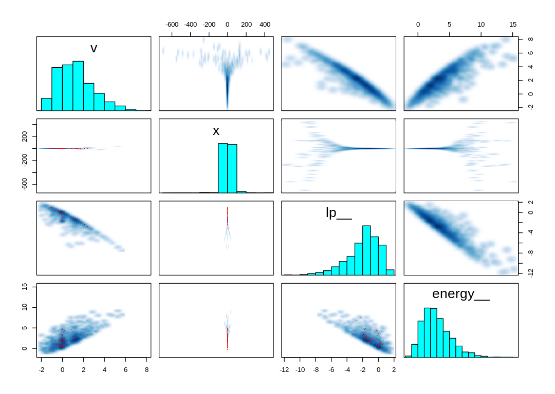
This model produces warnings even producing the pairs() plot:
iplot(function() {
  pairs(m13.7@stanfit)
})
iplot(function() {
  traceplot(m13.7)
}, ar=2)
[1] 1000
[1] 1
[1] 1000
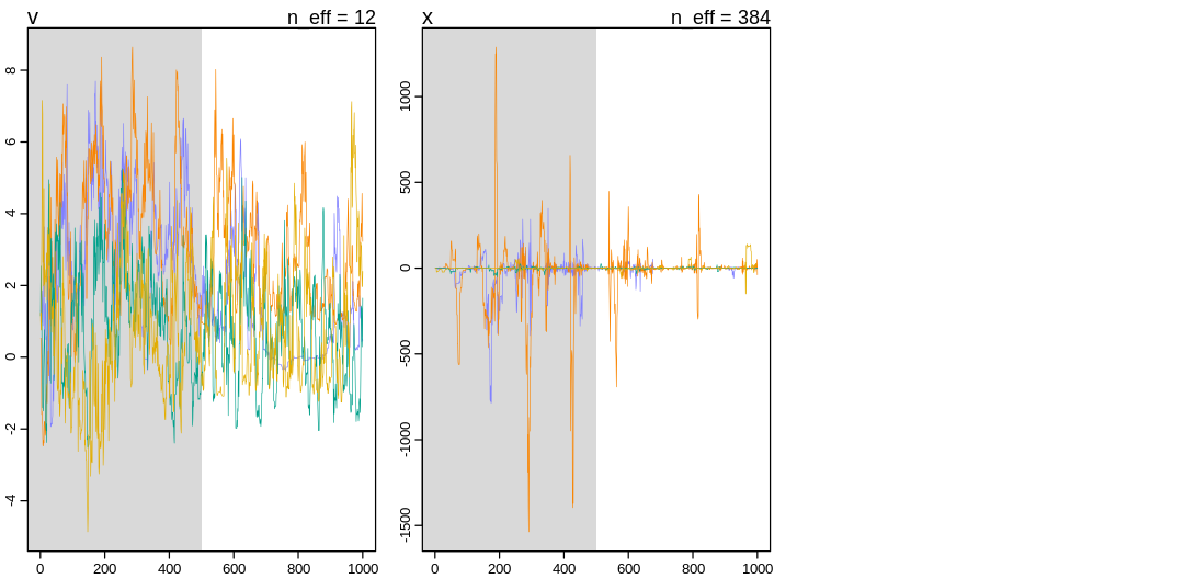
Unlike the pairs() plot from the Funnel, the divergent transitions produced by the Cauchy
distribution are not associated with steep contours.
Let’s at least attempt to reparameterize the model to confirm whether or not it will help. One way to think about reparameterizing a model is as factoring the quantile function. As explained in Quantile function, a sample from a given distribution may be obtained in principle by applying its quantile function to a sample from a uniform distribution. The quantile function for the Normal distribution is:
So for the standard normal: $\( Q_s(p) = \sqrt{2} \cdot erf^{-1} (2p - 1) \)$
Imagining p comes from a uniform distribution in both cases, we can write:
$\(
Q(p, \mu, \sigma) = \mu + \sigma Q_s(p)
\)$
Starting from the quantile function for the Cauchy distribution: $\( Q(p, x_0, \gamma) = x_0 + \gamma \tan[\pi(p - \frac{1}{2})] \)$
Define the standard Cauchy distribution quantile function as: $\( Q_s(p) = \tan[\pi(p - \frac{1}{2})] \)$
So that: $\( Q(p, x_0, \gamma) = x_0 + \gamma Q_s(p) \)$
Finally, define a new non-centered model: $\( \begin{align} S_i & \sim Binomial(N_i,p_i) \\ logit(p_i) & = \alpha + \sigma \cdot a_{tank[i]} \\ a_{tank} & \sim Cauchy(0, 1), tank = 1..48 \\ \alpha & \sim Normal(0, 1) \\ \sigma & \sim Exponential(1) \\ \end{align} \)$
Unfortunately, this model produces the same divergent transitions:
m_tank_noncen_cauchy <- ulam(
  alist(
    S ~ dbinom(N, p),
    logit(p) <- a_bar + sigma * std_c[tank],
    std_c[tank] ~ dcauchy(0, 1),
    a_bar ~ dnorm(0, 1),
    sigma ~ dexp(1)
  ),
  data = rf_dat, chains = 4, cores = 4, log_lik = TRUE
)
Warning message:
“There were 175 divergent transitions after warmup. See
https://mc-stan.org/misc/warnings.html#divergent-transitions-after-warmup
to find out why this is a problem and how to eliminate them.”
Warning message:
“Examine the pairs() plot to diagnose sampling problems
”
Warning message:
“Bulk Effective Samples Size (ESS) is too low, indicating posterior means and medians may be unreliable.
Running the chains for more iterations may help. See
https://mc-stan.org/misc/warnings.html#bulk-ess”
Warning message:
“Tail Effective Samples Size (ESS) is too low, indicating posterior variances and tail quantiles may be unreliable.
Running the chains for more iterations may help. See
https://mc-stan.org/misc/warnings.html#tail-ess”
What’s more likely going on here is that the energy sanity checks in MCMC are too tight for the
extreme deviates produced by the Cauchy distribution. Consider the quantile function for the Cauchy
distribution above, defined based on the trigonometric tan function. This definition leads to
extreme negative or positive deviates when p is near either zero or one; notice this term
approaches negative infinity as p approaches zero and positive infinity as it approaches one.
Notice in the pairs() plot above, the trace plot, and in the number of effective samples that
larger parameters like a[38] are harder to sample than a[41]. Part of the reason for this may
be that these samples would get rejected as divergent transitions, even when we rarely happen to
sample from this part of the posterior.
In the posterior distributions parameter a[38] is much less certain than a[41]. In the original
and Cauchy model, parameter 38 is inferred to be larger than 41. All large parameters are going to
be more uncertain with the Cauchy distribution and in fact for all distributions with a thick tail;
getting a sample of a large value implies a rather large deviate from the distribution and a
specific large deviate is relatively unlikely relative to other large deviates (the long tail is
relatively flat). Additionally, a large observation could be explained by applying a larger range of
parameters to a distribution because every parameterization has large tails that allow for the
observation. The same observation could be made of the Student-t inferences in the next question.
The increase in uncertainty for larger parameters exists even in model m13.2 but is much more
significant for thick-tailed distributions.
display(precis(m_tank_cauchy, depth = 2), mimetypes="text/plain")
iplot(function() {
  plot(precis(m_tank_cauchy, depth=2), main='m_tank_cauchy')
}, ar=1.0)
      mean        sd        5.5%        94.5%        n_eff     Rhat4
a[1]   2.02074871 0.9071214  0.85242700  3.591473539  918.9857 1.0009173
a[2]   5.08063539 5.6135330  1.47001998 15.529967462  184.0237 1.0202038
a[3]   1.08871877 0.6087445  0.09970443  2.050928888 1914.7659 0.9991960
a[4]   5.34806778 5.3096227  1.42600693 14.731180562  219.9149 1.0165869
a[5]   2.00126467 0.8075904  0.89882000  3.349092010 1100.8160 1.0017914
a[6]   1.98253983 0.7965357  0.91012950  3.358615146 1335.3333 1.0032704
a[7]   5.48352961 6.0275677  1.47545212 17.462532440  224.3699 1.0176450
a[8]   2.04565548 0.9223549  0.81531533  3.692914583 1276.6374 1.0003314
a[9]  -0.06670843 0.6941407 -1.20520326  0.975139514 2268.3708 1.0001835
a[10]  1.98579817 0.8241046  0.87315244  3.398005489 1578.1110 1.0001169
a[11]  1.10219059 0.6000629  0.13711057  2.058647278 1976.7846 0.9996361
a[12]  0.71705090 0.6215530 -0.29810360  1.724685854 2206.2297 0.9984469
a[13]  1.07690149 0.5836904  0.14492897  1.991944805 1911.2428 0.9987297
a[14]  0.36407700 0.6333418 -0.68138877  1.363754476 2010.1528 1.0004197
a[15]  2.00523689 0.8558858  0.85532012  3.528721252 1382.2451 1.0027034
a[16]  2.00888444 0.8580599  0.88866106  3.475468341 1464.6589 0.9992135
a[17]  2.90577874 0.9909286  1.66172262  4.720532096  735.4820 1.0072523
a[18]  2.26929680 0.6271743  1.37341215  3.386935343 1667.9526 1.0008504
a[19]  1.91587034 0.5412981  1.15417804  2.842269103 1979.8679 1.0024365
a[20]  7.46488936 6.4006676  2.33103400 20.434842057  276.1079 1.0054083
a[21]  2.24510772 0.6552339  1.33715641  3.388647320 1818.0964 0.9995491
a[22]  2.25944660 0.6180430  1.37336120  3.319773411 1688.4116 1.0012850
a[23]  2.25705075 0.6554530  1.36246595  3.380442895 1260.6602 0.9991668
a[24]  1.65900394 0.4989366  0.94952787  2.512699565 2222.7083 0.9984226
a[25] -1.05131200 0.4834173 -1.83872058 -0.303219247 2329.3534 1.0020294
a[26]  0.25188241 0.4271093 -0.42990295  0.937043069 2549.8136 0.9983111
a[27] -1.56126970 0.5249921 -2.43224094 -0.761120978 2685.1380 0.9990867
a[28] -0.44590070 0.4309351 -1.15550868  0.245554674 2377.9549 0.9994350
a[29]  0.25599516 0.4244766 -0.42782030  0.932784716 1828.0068 0.9987739
a[30]  1.44085476 0.4416018  0.76392535  2.155465105 1949.3210 0.9990049
a[31] -0.63029760 0.4108380 -1.29041702 -0.006518082 2665.1562 1.0010634
a[32] -0.27100654 0.4232400 -0.96023605  0.419768856 2247.8276 0.9997774
a[33]  3.22262938 0.9973633  1.94834313  4.959556218 1396.5489 1.0020735
a[34]  2.56972242 0.6701889  1.62675923  3.741053054 1736.6982 0.9989668
a[35]  2.56777345 0.6490009  1.69929537  3.694454406 1739.0035 0.9994178
a[36]  1.96570383 0.4858548  1.23301259  2.819460114 2012.4684 1.0015704
a[37]  1.98799694 0.5035797  1.23037122  2.836648876 2001.3305 0.9994696
a[38]  8.02495538 6.0751137  2.81137423 20.039817681  311.5927 1.0088157
a[39]  2.58042809 0.6652044  1.62420833  3.721778372 1610.4960 1.0015275
a[40]  2.23896780 0.5512907  1.45957120  3.194526254 1802.0274 1.0013133
a[41] -1.97976981 0.5132851 -2.82647735 -1.194158470 2876.1564 0.9999574
a[42] -0.57033631 0.3421285 -1.08923720 -0.027005564 2383.8508 0.9995389
a[43] -0.44529294 0.3518008 -1.03074350  0.094351028 2186.5462 0.9992146
a[44] -0.31576376 0.3524630 -0.88843056  0.255641167 2215.4965 0.9989419
a[45]  0.65019851 0.3629227  0.06478948  1.226211498 2387.6183 0.9985297
a[46] -0.56214731 0.3553647 -1.13696510  0.001795373 1767.3904 1.0018065
a[47]  1.97943131 0.4780286  1.28626116  2.824255982 1515.1132 1.0004457
a[48]  0.02712795 0.3567742 -0.54605395  0.608807470 2698.3412 0.9999105
a_bar  1.40921335 0.2954609  0.92210858  1.889850620 1365.0294 0.9998429
sigma  1.02266302 0.2299454  0.68944188  1.418096533 1436.4947 0.9992479
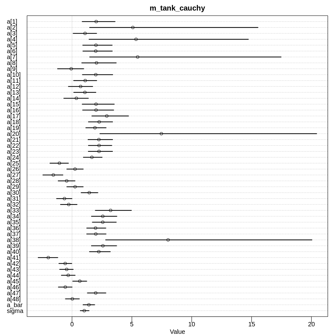
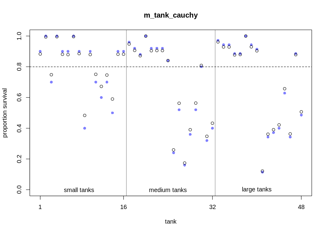
The same trends in shrinkage exist in this model as the original model. Because of the thicker tails, the model doesn’t apply as much shrinkage to extreme observations. Because of the difficulty in sampling, the shrinkage is more variable.
post <- extract.samples(m_tank_cauchy)
plot_means(post, "m_tank_cauchy")
13M4. Now use a Student-t distribution with \(\nu = 2\) for the intercepts:
Refer back to the Student-t example in Chapter 7 (page 234), if necessary. Compare the resulting posterior to both the original model and the Cauchy model in 13M3. Can you explain the differences and similarities in shrinkage in terms of the properties of these distributions?
Answer. This model produces some but fewer divergent transitions, likely because of deviates coming from the thick tails:
m_tank_student_t <- ulam(
  alist(
    S ~ dbinom(N, p),
    logit(p) <- a[tank],
    a[tank] ~ dstudent(2, a_bar, sigma),
    a_bar ~ dnorm(0, 1),
    sigma ~ dexp(1)
  ),
  data = rf_dat, chains = 4, cores = 4, log_lik = TRUE
)
Warning message:
“There were 23 divergent transitions after warmup. See
https://mc-stan.org/misc/warnings.html#divergent-transitions-after-warmup
to find out why this is a problem and how to eliminate them.”
Warning message:
“Examine the pairs() plot to diagnose sampling problems
”
Warning message:
“Tail Effective Samples Size (ESS) is too low, indicating posterior variances and tail quantiles may be unreliable.
Running the chains for more iterations may help. See
https://mc-stan.org/misc/warnings.html#tail-ess”
Although we won’t address these divergent transitions, let’s at least check how much mixing is occurring:
iplot(function() {
  pairs(m_tank_cauchy@stanfit, pars=sel_pars)
})
iplot(function() {
  traceplot(m_tank_cauchy, pars=sel_pars)
}, ar=2)

display(precis(m_tank_student_t, depth = 2), mimetypes="text/plain")
iplot(function() {
  plot(precis(m_tank_student_t, depth=2), main='m_tank_student_t')
}, ar=1.0)
[1] 1000
[1] 1
[1] 1000
      mean        sd        5.5%         94.5%        n_eff     Rhat4
a[1]   2.04725655 0.8778747  0.871823859  3.647687960 2122.6056 1.0003399
a[2]   3.90473622 2.9777343  1.446281475  8.510423620  191.4751 1.0244580
a[3]   1.04326429 0.6553285  0.005875528  2.117972525 2643.9504 0.9992451
a[4]   3.95410367 3.2294508  1.441470395  8.729328164  400.5191 1.0105738
a[5]   2.06750080 0.8922228  0.831528014  3.532404509 1902.0670 0.9988724
a[6]   2.02938741 0.8439318  0.814034020  3.503880965 2468.8427 0.9994303
a[7]   4.15625592 3.4024650  1.426585935 10.235777065  361.9207 1.0170703
a[8]   2.06774019 0.8632288  0.877024267  3.556407188 1597.3054 1.0009802
a[9]  -0.10462965 0.6578048 -1.121308896  0.946081009 3026.3025 0.9993105
a[10]  2.04314549 0.8892821  0.837122342  3.547323152 2126.3912 0.9997456
a[11]  1.04140780 0.6379525  0.064567383  2.021032767 2653.8252 0.9999189
a[12]  0.65995294 0.6552864 -0.365900237  1.702378295 3946.9351 0.9987835
a[13]  1.04225564 0.6523299  0.007343597  2.057120476 3652.7492 0.9990539
a[14]  0.28639782 0.6146079 -0.698686621  1.266751133 4002.0900 0.9989735
a[15]  2.04128604 0.8446250  0.861431611  3.589458757 2711.0927 0.9997029
a[16]  2.06334685 0.9013063  0.905839046  3.537639739 1200.6666 0.9996603
a[17]  2.89133936 0.9371686  1.671942562  4.477336754  773.6690 1.0041677
a[18]  2.29857640 0.6648269  1.343919113  3.418462504 2464.5341 0.9988470
a[19]  1.93156660 0.5585599  1.126782621  2.863646838 3296.2132 0.9994535
a[20]  5.36604144 4.5193363  2.288434355 11.584606975  133.5962 1.0401715
a[21]  2.30514991 0.6389253  1.422428884  3.396027753 2637.1596 1.0009236
a[22]  2.32934339 0.6848534  1.352722042  3.547294683 1869.0926 0.9990927
a[23]  2.28287074 0.6400545  1.341220247  3.391660581 3108.9502 1.0010721
a[24]  1.66844553 0.4730304  0.936662732  2.435130302 3249.9024 0.9986294
a[25] -1.02181146 0.4604636 -1.755834917 -0.289828566 3844.8723 0.9987312
a[26]  0.20469347 0.3915170 -0.400534652  0.828131111 4221.5758 0.9985146
a[27] -1.54062058 0.5531033 -2.489548491 -0.695332412 3297.7432 0.9999920
a[28] -0.45251544 0.4113042 -1.126430537  0.184855521 4465.5235 0.9989616
a[29]  0.19661006 0.3996425 -0.443711289  0.818053312 2839.5558 0.9996762
a[30]  1.45412325 0.4875788  0.708497099  2.259780387 3652.2842 1.0002202
a[31] -0.62720249 0.4390594 -1.353746964  0.065525897 3483.0887 0.9997379
a[32] -0.28161310 0.3942326 -0.923826504  0.345727707 4226.1389 0.9990332
a[33]  3.23692186 0.8950969  2.042190788  4.860836724 1838.0201 0.9992302
a[34]  2.65219664 0.6715726  1.713431690  3.798236076 2098.1268 0.9994387
a[35]  2.64065964 0.6318227  1.732946261  3.755456530 3084.5518 0.9983295
a[36]  1.99961969 0.5124537  1.251753594  2.824701731 3125.8326 0.9991991
a[37]  2.00861682 0.4934536  1.270701241  2.848163204 3154.5929 0.9991247
a[38]  5.58947800 3.5324878  2.641857926 11.554274691  481.9251 1.0037527
a[39]  2.63428729 0.6582212  1.710314715  3.760783921 2605.4197 0.9994242
a[40]  2.27262382 0.5402218  1.451764695  3.160739319 2227.1285 1.0004352
a[41] -1.95920729 0.5280561 -2.833271219 -1.189589735 3167.4333 0.9996033
a[42] -0.56667988 0.3555039 -1.166659356 -0.012356600 4790.1770 0.9984502
a[43] -0.44304685 0.3638038 -1.019214656  0.133621238 4070.1635 0.9986671
a[44] -0.30835693 0.3409142 -0.854523120  0.218789628 3428.1564 0.9986899
a[45]  0.62574264 0.3277412  0.121233841  1.156075731 3833.7581 0.9987596
a[46] -0.55968437 0.3572011 -1.133322881  0.004806139 4086.7395 1.0002365
a[47]  2.01710885 0.5016654  1.276360950  2.879223182 3419.5396 0.9993304
a[48]  0.02400507 0.3515067 -0.523944423  0.585838566 4096.6480 0.9990067
a_bar  1.34056986 0.2636477  0.920039770  1.741106783 2304.0602 1.0009423
sigma  1.26496733 0.2341194  0.935199795  1.649668863 1732.1119 1.0033691
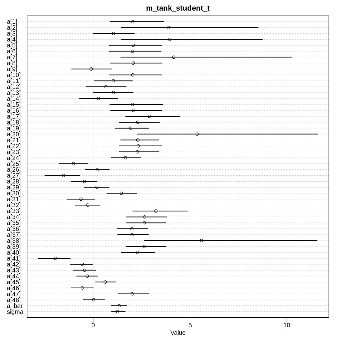
Similar trends in shrinkage exist in this model. Because of the thicker tails, the model doesn’t apply as much shrinkage to extreme observations. Improved sampling relative to the Cauchy distribution seems to have produced slightly more consistent shrinkage.
post <- extract.samples(m_tank_student_t)
plot_means(post, "m_tank_student_t")
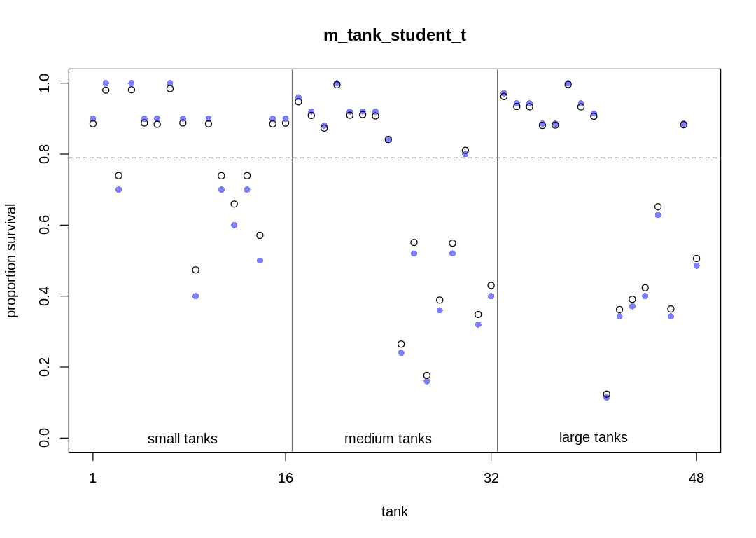
13M5. Modify the cross-classified chimpanzees model m13.4 so that the adaptive prior for
blocks contains a parameter \(\gamma\) for its mean:
Compare this model to m13.4. What has including \(\gamma\) done?
Answer. First, let’s reproduce the relevant plots from the chapter:
data(chimpanzees)
d <- chimpanzees
d$treatment <- 1 + d$prosoc_left + 2 * d$condition

dat_list <- list(
  pulled_left = d$pulled_left,
  actor = d$actor,
  block_id = d$block,
  treatment = as.integer(d$treatment)
)

set.seed(13)
m13.4 <- ulam(
  alist(
    pulled_left ~ dbinom(1, p),
    logit(p) <- a[actor] + g[block_id] + b[treatment],
    b[treatment] ~ dnorm(0, 0.5),
    ## adaptive priors
    a[actor] ~ dnorm(a_bar, sigma_a),
    g[block_id] ~ dnorm(0, sigma_g),
    ## hyper-priors
    a_bar ~ dnorm(0, 1.5),
    sigma_a ~ dexp(1),
    sigma_g ~ dexp(1)
  ),
  data = dat_list, chains = 4, cores = 4, log_lik = TRUE
)

display(precis(m13.4, depth = 2), mimetypes="text/plain")
iplot(function() {
  plot(precis(m13.4, depth=2), main='m13.4')
}, ar=2.0)
Warning message:
“There were 8 divergent transitions after warmup. See
https://mc-stan.org/misc/warnings.html#divergent-transitions-after-warmup
to find out why this is a problem and how to eliminate them.”
Warning message:
“Examine the pairs() plot to diagnose sampling problems
”
Warning message:
“Bulk Effective Samples Size (ESS) is too low, indicating posterior means and medians may be unreliable.
Running the chains for more iterations may help. See
https://mc-stan.org/misc/warnings.html#bulk-ess”
Warning message:
“Tail Effective Samples Size (ESS) is too low, indicating posterior variances and tail quantiles may be unreliable.
Running the chains for more iterations may help. See
https://mc-stan.org/misc/warnings.html#tail-ess”
        mean        sd        5.5%         94.5%       n_eff    Rhat4
b[1]    -0.11615950 0.3005730 -0.590557431  0.35487909 341.9669 1.013459
b[2]     0.39798057 0.3082406 -0.091243273  0.89572497 382.5939 1.008442
b[3]    -0.46319143 0.3074857 -0.955775110  0.02294964 442.0306 1.008027
b[4]     0.29072509 0.3022209 -0.198956418  0.77520474 340.5103 1.005458
a[1]    -0.37237534 0.3735216 -0.952143414  0.24461789 360.9980 1.005206
a[2]     4.64362246 1.2404897  3.062224463  6.73789096 677.9918 1.012002
a[3]    -0.68062851 0.3697046 -1.272373182 -0.08899088 286.9193 1.005228
a[4]    -0.67622831 0.3732220 -1.236789673 -0.06893589 371.2960 1.007441
a[5]    -0.35994244 0.3656058 -0.921735209  0.25147471 354.5740 1.007732
a[6]     0.57366442 0.3809162 -0.004217109  1.17408617 325.9938 1.012455
a[7]     2.09973745 0.4622194  1.398033779  2.83875730 431.2037 1.006421
g[1]    -0.18166155 0.2473370 -0.672918642  0.08538534 225.9254 1.014807
g[2]     0.03786340 0.1936058 -0.230668997  0.35845635 410.2488 1.014838
g[3]     0.05187367 0.1948952 -0.216316191  0.38606310 389.5636 1.021056
g[4]     0.01162107 0.1920499 -0.286063273  0.31457637 444.1353 1.010494
g[5]    -0.03372976 0.1875264 -0.327363879  0.23893233 312.3261 1.014771
g[6]     0.11314564 0.2052871 -0.139423515  0.48303072 419.7813 1.017376
a_bar    0.55787921 0.7133251 -0.526962103  1.69749820 557.0130 1.008263
sigma_a  2.03959649 0.6769575  1.216298295  3.40139094 312.7584 1.008526
sigma_g  0.22291426 0.1816101  0.021827743  0.54077837 160.8728 1.024422
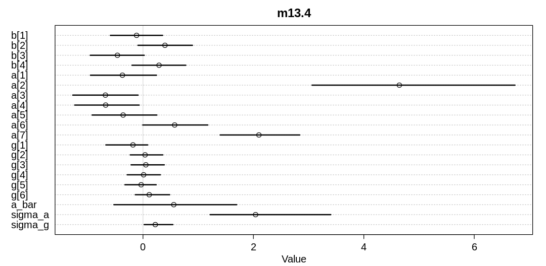
When we add the new parameter, the number of divergent transitions increase:
m13.4_extra_param <- ulam(
  alist(
    pulled_left ~ dbinom(1, p),
    logit(p) <- a[actor] + g[block_id] + b[treatment],
    b[treatment] ~ dnorm(0, 0.5),
    ## adaptive priors
    a[actor] ~ dnorm(a_bar, sigma_a),
    g[block_id] ~ dnorm(g_bar, sigma_g),
    ## hyper-priors
    a_bar ~ dnorm(0, 1.5),
    g_bar ~ dnorm(0, 1.5),
    sigma_a ~ dexp(1),
    sigma_g ~ dexp(1)
  ),
  data = dat_list, chains = 4, cores = 4, log_lik = TRUE
)
Warning message:
“There were 385 divergent transitions after warmup. See
https://mc-stan.org/misc/warnings.html#divergent-transitions-after-warmup
to find out why this is a problem and how to eliminate them.”
Warning message:
“Examine the pairs() plot to diagnose sampling problems
”
Warning message:
“The largest R-hat is 1.55, indicating chains have not mixed.
Running the chains for more iterations may help. See
https://mc-stan.org/misc/warnings.html#r-hat”
Warning message:
“Bulk Effective Samples Size (ESS) is too low, indicating posterior means and medians may be unreliable.
Running the chains for more iterations may help. See
https://mc-stan.org/misc/warnings.html#bulk-ess”
Warning message:
“Tail Effective Samples Size (ESS) is too low, indicating posterior variances and tail quantiles may be unreliable.
Running the chains for more iterations may help. See
https://mc-stan.org/misc/warnings.html#tail-ess”
We also see many HDPI increase:
display(precis(m13.4_extra_param, depth = 2), mimetypes="text/plain")
iplot(function() {
  plot(precis(m13.4_extra_param, depth=2), main='m13.4_extra_param')
}, ar=2.0)
        mean        sd        5.5%        94.5%       n_eff      Rhat4
b[1]    -0.17813736 0.2603696 -0.59177498  0.28168289 477.802182 1.020488
b[2]     0.26875222 0.3289717 -0.10305314  0.83007340   5.189463 1.300721
b[3]    -0.58919595 0.3080753 -0.92700257 -0.07270346   6.211768 1.236896
b[4]     0.18286977 0.2936379 -0.16282659  0.69268802  10.554156 1.144322
a[1]    -0.49538280 1.0579117 -2.39711975  0.79275830  10.970626 1.147074
a[2]     4.83839506 1.7132034  2.07716453  6.98893009   6.084632 1.258717
a[3]    -0.64527672 1.1988423 -2.64370490  0.72398162   5.102209 1.310564
a[4]    -0.76862008 1.0822653 -2.67498627  0.44261506   8.237649 1.191341
a[5]    -0.36943430 1.1816639 -2.38146859  1.04030622   5.514536 1.294735
a[6]     0.33962335 0.9951733 -1.49753082  1.71581973  43.629054 1.067636
a[7]     2.01019961 1.0936865  0.01590190  3.31309956   9.062989 1.164873
g[1]     0.07292304 0.9791712 -1.19950901  1.82572130  48.922049 1.080038
g[2]     0.23335141 0.9991374 -0.98702361  2.01905031  16.150120 1.120425
g[3]     0.25257601 1.0100317 -0.94932471  2.01178480  15.123122 1.122954
g[4]     0.21687297 1.0027637 -1.02863119  1.98399979  17.569246 1.114660
g[5]     0.18323217 0.9935132 -1.03603191  1.96190655  19.472040 1.105377
g[6]     0.29531996 1.0254596 -0.88359120  2.13254755  12.467377 1.133592
a_bar    0.34393322 0.9656677 -1.34241524  1.81217244 289.944388 1.023295
g_bar    0.20735506 0.9933946 -1.02400712  1.97511367  17.496528 1.113645
sigma_a  1.97322416 0.5484229  1.27586783  3.04137557 707.275121 1.016221
sigma_g  0.17771181 0.1706753  0.01894145  0.49719091   6.824275 1.220724
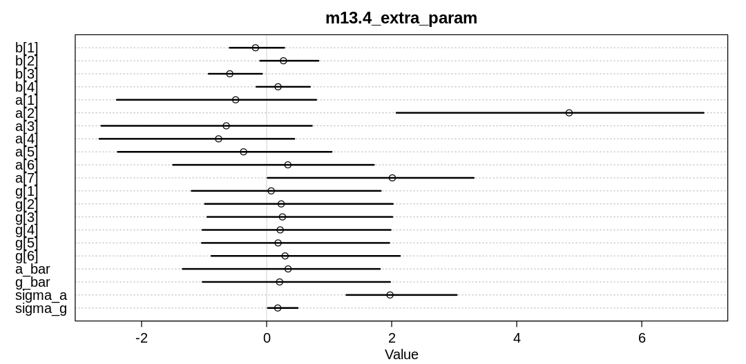
Notice the previously specified prior for the new parameter \(\bar{\gamma}\) did not change significantly in the posterior. Let’s change the prior to: $\( \bar{\gamma} \sim Normal(5, 4) \)$
With this change, we can come up with significantly different inferences:
m13.4_extra_param_new_prior <- ulam(
  alist(
    pulled_left ~ dbinom(1, p),
    logit(p) <- a[actor] + g[block_id] + b[treatment],
    b[treatment] ~ dnorm(0, 0.5),
    ## adaptive priors
    a[actor] ~ dnorm(a_bar, sigma_a),
    g[block_id] ~ dnorm(g_bar, sigma_g),
    ## hyper-priors
    a_bar ~ dnorm(0, 1.5),
    g_bar ~ dnorm(5, 1.5),
    sigma_a ~ dexp(1),
    sigma_g ~ dexp(1)
  ),
  data = dat_list, chains = 4, cores = 4, log_lik = TRUE
)

display(precis(m13.4_extra_param_new_prior, depth = 2), mimetypes="text/plain")
iplot(function() {
  plot(precis(m13.4_extra_param_new_prior, depth=2), main='m13.4_extra_param_new_prior')
}, ar=2.0)
Warning message:
“There were 42 divergent transitions after warmup. See
https://mc-stan.org/misc/warnings.html#divergent-transitions-after-warmup
to find out why this is a problem and how to eliminate them.”
Warning message:
“There were 171 transitions after warmup that exceeded the maximum treedepth. Increase max_treedepth above 10. See
https://mc-stan.org/misc/warnings.html#maximum-treedepth-exceeded”
Warning message:
“Examine the pairs() plot to diagnose sampling problems
”
Warning message:
“Bulk Effective Samples Size (ESS) is too low, indicating posterior means and medians may be unreliable.
Running the chains for more iterations may help. See
https://mc-stan.org/misc/warnings.html#bulk-ess”
Warning message:
“Tail Effective Samples Size (ESS) is too low, indicating posterior variances and tail quantiles may be unreliable.
Running the chains for more iterations may help. See
https://mc-stan.org/misc/warnings.html#tail-ess”
        mean       sd        5.5%        94.5%       n_eff    Rhat4
b[1]    -0.1982002 0.3104625 -0.72790681  0.29152455 647.2476 1.000009
b[2]     0.3332580 0.3027702 -0.15706229  0.80377376 557.5257 1.001001
b[3]    -0.5483467 0.3068423 -1.05140473 -0.05345565 705.2644 1.002405
b[4]     0.2159099 0.3072428 -0.28113841  0.71039389 726.5421 1.000120
a[1]    -3.5701226 1.2542313 -5.56103644 -1.66419461 148.8309 1.029586
a[2]     1.8570795 1.8344063 -0.81761566  5.02372101 275.7184 1.008268
a[3]    -3.8649515 1.2612236 -5.88895760 -1.97150792 149.4719 1.027678
a[4]    -3.8609477 1.2726703 -5.92074520 -1.91772504 149.9519 1.028724
a[5]    -3.5654391 1.2710183 -5.55586118 -1.66868112 146.0176 1.029502
a[6]    -2.6169841 1.2572365 -4.64793820 -0.68266901 145.9102 1.029996
a[7]    -1.0728047 1.2963241 -3.22741473  0.85734865 153.0102 1.025513
g[1]     3.1049763 1.2554391  1.13769846  5.07737529 139.8131 1.034503
g[2]     3.3204328 1.2509203  1.32067650  5.25879070 143.7018 1.028116
g[3]     3.3377147 1.2520669  1.35748335  5.28192803 143.3000 1.027749
g[4]     3.2873947 1.2514220  1.29297229  5.27030263 142.4782 1.030420
g[5]     3.2420809 1.2593901  1.24941038  5.19733086 144.4855 1.031121
g[6]     3.3967067 1.2540103  1.41208240  5.35444757 146.0944 1.026500
a_bar   -1.8202624 1.2145033 -3.79149760  0.10998530 232.1819 1.016298
g_bar    3.2892587 1.2428016  1.33463476  5.24329650 142.9446 1.029420
sigma_a  2.2105176 0.7628012  1.26305682  3.55048611 643.9483 1.007105
sigma_g  0.2233260 0.1670153  0.05083342  0.52403040 374.7944 1.018752
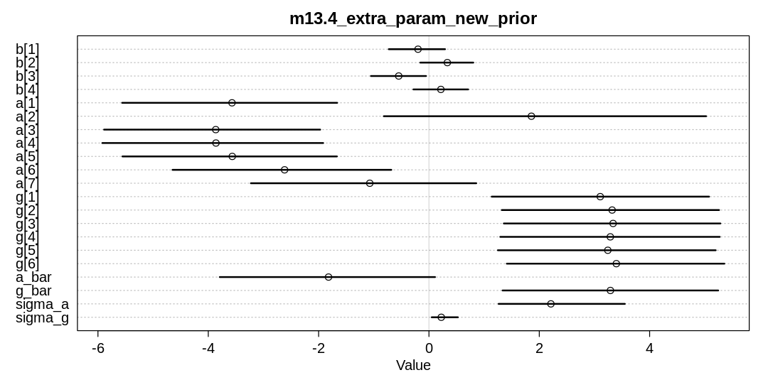
All these symptoms are indicative of a non-identifiable parameter, as discussed in the chapter at the start of section 13.3.1. We encountered the same issue in question 13M1.
ERROR:
Likewise, the tails of distributions strongly influence can (sic) outliers are shrunk or not towards the mean.
Likewise, the tails of distributions strongly influence whether outliers are shrunk towards the mean.
13M6. Sometimes the prior and the data (through the likelihood) are in conflict, because they concentrate around different regions of parameter space. What happens in these cases depends a lot upon the shape of the tails of the distributions. Likewise, the tails of distributions strongly influence can outliers are shrunk or not towards the mean. I want you to consider four different models to fit to one observation at \(y = 0\). The models differ only in the distributions assigned to the likelihood and the prior. Here are the four models:
Model NN: $\( \begin{align} y & \sim Normal(\mu, 1) \\ \mu & \sim Normal(10, 1) \end{align} \)$
Model TN: $\( \begin{align} y & \sim Student(2, \mu, 1) \\ \mu & \sim Normal(10, 1) \end{align} \)$
Model NT: $\( \begin{align} y & \sim Normal(\mu, 1) \\ \mu & \sim Student(2, 10, 1) \end{align} \)$
Model TT: $\( \begin{align} y & \sim Student(2, \mu, 1) \\ \mu & \sim Student(2, 10, 1) \end{align} \)$
Estimate the posterior distributions for these models and compare them. Can you explain the results, using the properties of the distributions?
Answer. Fit model NN:
m_nn <- ulam(
  alist(
    y ~ dnorm(mu, 1),
    mu ~ dnorm(10, 1)
  ),
  data = list(y = 0), chains = 4
)
flush.console()
SAMPLING FOR MODEL '143b90eac39af089032ce5f1b377f41a' NOW (CHAIN 1).
Chain 1:
Chain 1: Gradient evaluation took 6e-06 seconds
Chain 1: 1000 transitions using 10 leapfrog steps per transition would take 0.06 seconds.
Chain 1: Adjust your expectations accordingly!
Chain 1:
Chain 1:
Chain 1: Iteration:   1 / 1000 [  0%]  (Warmup)
Chain 1: Iteration: 100 / 1000 [ 10%]  (Warmup)
Chain 1: Iteration: 200 / 1000 [ 20%]  (Warmup)
Chain 1: Iteration: 300 / 1000 [ 30%]  (Warmup)
Chain 1: Iteration: 400 / 1000 [ 40%]  (Warmup)
Chain 1: Iteration: 500 / 1000 [ 50%]  (Warmup)
Chain 1: Iteration: 501 / 1000 [ 50%]  (Sampling)
Chain 1: Iteration: 600 / 1000 [ 60%]  (Sampling)
Chain 1: Iteration: 700 / 1000 [ 70%]  (Sampling)
Chain 1: Iteration: 800 / 1000 [ 80%]  (Sampling)
Chain 1: Iteration: 900 / 1000 [ 90%]  (Sampling)
Chain 1: Iteration: 1000 / 1000 [100%]  (Sampling)
Chain 1:
Chain 1:  Elapsed Time: 0.004895 seconds (Warm-up)
Chain 1:                0.004482 seconds (Sampling)
Chain 1:                0.009377 seconds (Total)
Chain 1:

SAMPLING FOR MODEL '143b90eac39af089032ce5f1b377f41a' NOW (CHAIN 2).
Chain 2:
Chain 2: Gradient evaluation took 3e-06 seconds
Chain 2: 1000 transitions using 10 leapfrog steps per transition would take 0.03 seconds.
Chain 2: Adjust your expectations accordingly!
Chain 2:
Chain 2:
Chain 2: Iteration:   1 / 1000 [  0%]  (Warmup)
Chain 2: Iteration: 100 / 1000 [ 10%]  (Warmup)
Chain 2: Iteration: 200 / 1000 [ 20%]  (Warmup)
Chain 2: Iteration: 300 / 1000 [ 30%]  (Warmup)
Chain 2: Iteration: 400 / 1000 [ 40%]  (Warmup)
Chain 2: Iteration: 500 / 1000 [ 50%]  (Warmup)
Chain 2: Iteration: 501 / 1000 [ 50%]  (Sampling)
Chain 2: Iteration: 600 / 1000 [ 60%]  (Sampling)
Chain 2: Iteration: 700 / 1000 [ 70%]  (Sampling)
Chain 2: Iteration: 800 / 1000 [ 80%]  (Sampling)
Chain 2: Iteration: 900 / 1000 [ 90%]  (Sampling)
Chain 2: Iteration: 1000 / 1000 [100%]  (Sampling)
Chain 2:
Chain 2:  Elapsed Time: 0.00465 seconds (Warm-up)
Chain 2:                0.004505 seconds (Sampling)
Chain 2:                0.009155 seconds (Total)
Chain 2:

SAMPLING FOR MODEL '143b90eac39af089032ce5f1b377f41a' NOW (CHAIN 3).
Chain 3:
Chain 3: Gradient evaluation took 2e-06 seconds
Chain 3: 1000 transitions using 10 leapfrog steps per transition would take 0.02 seconds.
Chain 3: Adjust your expectations accordingly!
Chain 3:
Chain 3:
Chain 3: Iteration:   1 / 1000 [  0%]  (Warmup)
Chain 3: Iteration: 100 / 1000 [ 10%]  (Warmup)
Chain 3: Iteration: 200 / 1000 [ 20%]  (Warmup)
Chain 3: Iteration: 300 / 1000 [ 30%]  (Warmup)
Chain 3: Iteration: 400 / 1000 [ 40%]  (Warmup)
Chain 3: Iteration: 500 / 1000 [ 50%]  (Warmup)
Chain 3: Iteration: 501 / 1000 [ 50%]  (Sampling)
Chain 3: Iteration: 600 / 1000 [ 60%]  (Sampling)
Chain 3: Iteration: 700 / 1000 [ 70%]  (Sampling)
Chain 3: Iteration: 800 / 1000 [ 80%]  (Sampling)
Chain 3: Iteration: 900 / 1000 [ 90%]  (Sampling)
Chain 3: Iteration: 1000 / 1000 [100%]  (Sampling)
Chain 3:
Chain 3:  Elapsed Time: 0.004714 seconds (Warm-up)
Chain 3:                0.00447 seconds (Sampling)
Chain 3:                0.009184 seconds (Total)
Chain 3:

SAMPLING FOR MODEL '143b90eac39af089032ce5f1b377f41a' NOW (CHAIN 4).
Chain 4:
Chain 4: Gradient evaluation took 2e-06 seconds
Chain 4: 1000 transitions using 10 leapfrog steps per transition would take 0.02 seconds.
Chain 4: Adjust your expectations accordingly!
Chain 4:
Chain 4:
Chain 4: Iteration:   1 / 1000 [  0%]  (Warmup)
Chain 4: Iteration: 100 / 1000 [ 10%]  (Warmup)
Chain 4: Iteration: 200 / 1000 [ 20%]  (Warmup)
Chain 4: Iteration: 300 / 1000 [ 30%]  (Warmup)
Chain 4: Iteration: 400 / 1000 [ 40%]  (Warmup)
Chain 4: Iteration: 500 / 1000 [ 50%]  (Warmup)
Chain 4: Iteration: 501 / 1000 [ 50%]  (Sampling)
Chain 4: Iteration: 600 / 1000 [ 60%]  (Sampling)
Chain 4: Iteration: 700 / 1000 [ 70%]  (Sampling)
Chain 4: Iteration: 800 / 1000 [ 80%]  (Sampling)
Chain 4: Iteration: 900 / 1000 [ 90%]  (Sampling)
Chain 4: Iteration: 1000 / 1000 [100%]  (Sampling)
Chain 4:
Chain 4:  Elapsed Time: 0.004569 seconds (Warm-up)
Chain 4:                0.003643 seconds (Sampling)
Chain 4:                0.008212 seconds (Total)
Chain 4:
Output of precis for model NN:
display(precis(m_nn), mimetypes="text/plain")
      result
mean    4.9778639
sd      0.6627867
5.5%    3.9302048
94.5%   6.0280244
n_eff 749.2425503
Rhat    1.0038182
Fit model TN:
m_tn <- ulam(
  alist(
    y ~ dstudent(2, mu, 1),
    mu ~ dnorm(10, 1)
  ),
  data = list(y = 0), chains = 4
)
flush.console()
SAMPLING FOR MODEL '63059b348951686cf386007a367cbbb4' NOW (CHAIN 1).
Chain 1:
Chain 1: Gradient evaluation took 5e-06 seconds
Chain 1: 1000 transitions using 10 leapfrog steps per transition would take 0.05 seconds.
Chain 1: Adjust your expectations accordingly!
Chain 1:
Chain 1:
Chain 1: Iteration:   1 / 1000 [  0%]  (Warmup)
Chain 1: Iteration: 100 / 1000 [ 10%]  (Warmup)
Chain 1: Iteration: 200 / 1000 [ 20%]  (Warmup)
Chain 1: Iteration: 300 / 1000 [ 30%]  (Warmup)
Chain 1: Iteration: 400 / 1000 [ 40%]  (Warmup)
Chain 1: Iteration: 500 / 1000 [ 50%]  (Warmup)
Chain 1: Iteration: 501 / 1000 [ 50%]  (Sampling)
Chain 1: Iteration: 600 / 1000 [ 60%]  (Sampling)
Chain 1: Iteration: 700 / 1000 [ 70%]  (Sampling)
Chain 1: Iteration: 800 / 1000 [ 80%]  (Sampling)
Chain 1: Iteration: 900 / 1000 [ 90%]  (Sampling)
Chain 1: Iteration: 1000 / 1000 [100%]  (Sampling)
Chain 1:
Chain 1:  Elapsed Time: 0.004073 seconds (Warm-up)
Chain 1:                0.004447 seconds (Sampling)
Chain 1:                0.00852 seconds (Total)
Chain 1:

SAMPLING FOR MODEL '63059b348951686cf386007a367cbbb4' NOW (CHAIN 2).
Chain 2:
Chain 2: Gradient evaluation took 3e-06 seconds
Chain 2: 1000 transitions using 10 leapfrog steps per transition would take 0.03 seconds.
Chain 2: Adjust your expectations accordingly!
Chain 2:
Chain 2:
Chain 2: Iteration:   1 / 1000 [  0%]  (Warmup)
Chain 2: Iteration: 100 / 1000 [ 10%]  (Warmup)
Chain 2: Iteration: 200 / 1000 [ 20%]  (Warmup)
Chain 2: Iteration: 300 / 1000 [ 30%]  (Warmup)
Chain 2: Iteration: 400 / 1000 [ 40%]  (Warmup)
Chain 2: Iteration: 500 / 1000 [ 50%]  (Warmup)
Chain 2: Iteration: 501 / 1000 [ 50%]  (Sampling)
Chain 2: Iteration: 600 / 1000 [ 60%]  (Sampling)
Chain 2: Iteration: 700 / 1000 [ 70%]  (Sampling)
Chain 2: Iteration: 800 / 1000 [ 80%]  (Sampling)
Chain 2: Iteration: 900 / 1000 [ 90%]  (Sampling)
Chain 2: Iteration: 1000 / 1000 [100%]  (Sampling)
Chain 2:
Chain 2:  Elapsed Time: 0.004472 seconds (Warm-up)
Chain 2:                0.004425 seconds (Sampling)
Chain 2:                0.008897 seconds (Total)
Chain 2:

SAMPLING FOR MODEL '63059b348951686cf386007a367cbbb4' NOW (CHAIN 3).
Chain 3:
Chain 3: Gradient evaluation took 3e-06 seconds
Chain 3: 1000 transitions using 10 leapfrog steps per transition would take 0.03 seconds.
Chain 3: Adjust your expectations accordingly!
Chain 3:
Chain 3:
Chain 3: Iteration:   1 / 1000 [  0%]  (Warmup)
Chain 3: Iteration: 100 / 1000 [ 10%]  (Warmup)
Chain 3: Iteration: 200 / 1000 [ 20%]  (Warmup)
Chain 3: Iteration: 300 / 1000 [ 30%]  (Warmup)
Chain 3: Iteration: 400 / 1000 [ 40%]  (Warmup)
Chain 3: Iteration: 500 / 1000 [ 50%]  (Warmup)
Chain 3: Iteration: 501 / 1000 [ 50%]  (Sampling)
Chain 3: Iteration: 600 / 1000 [ 60%]  (Sampling)
Chain 3: Iteration: 700 / 1000 [ 70%]  (Sampling)
Chain 3: Iteration: 800 / 1000 [ 80%]  (Sampling)
Chain 3: Iteration: 900 / 1000 [ 90%]  (Sampling)
Chain 3: Iteration: 1000 / 1000 [100%]  (Sampling)
Chain 3:
Chain 3:  Elapsed Time: 0.004509 seconds (Warm-up)
Chain 3:                0.003983 seconds (Sampling)
Chain 3:                0.008492 seconds (Total)
Chain 3:

SAMPLING FOR MODEL '63059b348951686cf386007a367cbbb4' NOW (CHAIN 4).
Chain 4:
Chain 4: Gradient evaluation took 2e-06 seconds
Chain 4: 1000 transitions using 10 leapfrog steps per transition would take 0.02 seconds.
Chain 4: Adjust your expectations accordingly!
Chain 4:
Chain 4:
Chain 4: Iteration:   1 / 1000 [  0%]  (Warmup)
Chain 4: Iteration: 100 / 1000 [ 10%]  (Warmup)
Chain 4: Iteration: 200 / 1000 [ 20%]  (Warmup)
Chain 4: Iteration: 300 / 1000 [ 30%]  (Warmup)
Chain 4: Iteration: 400 / 1000 [ 40%]  (Warmup)
Chain 4: Iteration: 500 / 1000 [ 50%]  (Warmup)
Chain 4: Iteration: 501 / 1000 [ 50%]  (Sampling)
Chain 4: Iteration: 600 / 1000 [ 60%]  (Sampling)
Chain 4: Iteration: 700 / 1000 [ 70%]  (Sampling)
Chain 4: Iteration: 800 / 1000 [ 80%]  (Sampling)
Chain 4: Iteration: 900 / 1000 [ 90%]  (Sampling)
Chain 4: Iteration: 1000 / 1000 [100%]  (Sampling)
Chain 4:
Chain 4:  Elapsed Time: 0.004659 seconds (Warm-up)
Chain 4:                0.004355 seconds (Sampling)
Chain 4:                0.009014 seconds (Total)
Chain 4:
Warning message:
“Tail Effective Samples Size (ESS) is too low, indicating posterior variances and tail quantiles may be unreliable.
Running the chains for more iterations may help. See
https://mc-stan.org/misc/warnings.html#tail-ess”
Output of precis for model TN:
display(precis(m_tn), mimetypes="text/plain")
      result
mean    9.731344
sd      1.029323
5.5%    8.098945
94.5%  11.393812
n_eff 530.009814
Rhat    1.008176
Fit model NT:
m_nt <- ulam(
  alist(
    y ~ dnorm(mu, 1),
    mu ~ dstudent(2, 10, 1)
  ),
  data = list(y = 0), chains = 4
)
flush.console()
SAMPLING FOR MODEL '5190f924283a6d1bedaa2b8ac8053620' NOW (CHAIN 1).
Chain 1:
Chain 1: Gradient evaluation took 7e-06 seconds
Chain 1: 1000 transitions using 10 leapfrog steps per transition would take 0.07 seconds.
Chain 1: Adjust your expectations accordingly!
Chain 1:
Chain 1:
Chain 1: Iteration:   1 / 1000 [  0%]  (Warmup)
Chain 1: Iteration: 100 / 1000 [ 10%]  (Warmup)
Chain 1: Iteration: 200 / 1000 [ 20%]  (Warmup)
Chain 1: Iteration: 300 / 1000 [ 30%]  (Warmup)
Chain 1: Iteration: 400 / 1000 [ 40%]  (Warmup)
Chain 1: Iteration: 500 / 1000 [ 50%]  (Warmup)
Chain 1: Iteration: 501 / 1000 [ 50%]  (Sampling)
Chain 1: Iteration: 600 / 1000 [ 60%]  (Sampling)
Chain 1: Iteration: 700 / 1000 [ 70%]  (Sampling)
Chain 1: Iteration: 800 / 1000 [ 80%]  (Sampling)
Chain 1: Iteration: 900 / 1000 [ 90%]  (Sampling)
Chain 1: Iteration: 1000 / 1000 [100%]  (Sampling)
Chain 1:
Chain 1:  Elapsed Time: 0.004228 seconds (Warm-up)
Chain 1:                0.004275 seconds (Sampling)
Chain 1:                0.008503 seconds (Total)
Chain 1:

SAMPLING FOR MODEL '5190f924283a6d1bedaa2b8ac8053620' NOW (CHAIN 2).
Chain 2:
Chain 2: Gradient evaluation took 3e-06 seconds
Chain 2: 1000 transitions using 10 leapfrog steps per transition would take 0.03 seconds.
Chain 2: Adjust your expectations accordingly!
Chain 2:
Chain 2:
Chain 2: Iteration:   1 / 1000 [  0%]  (Warmup)
Chain 2: Iteration: 100 / 1000 [ 10%]  (Warmup)
Chain 2: Iteration: 200 / 1000 [ 20%]  (Warmup)
Chain 2: Iteration: 300 / 1000 [ 30%]  (Warmup)
Chain 2: Iteration: 400 / 1000 [ 40%]  (Warmup)
Chain 2: Iteration: 500 / 1000 [ 50%]  (Warmup)
Chain 2: Iteration: 501 / 1000 [ 50%]  (Sampling)
Chain 2: Iteration: 600 / 1000 [ 60%]  (Sampling)
Chain 2: Iteration: 700 / 1000 [ 70%]  (Sampling)
Chain 2: Iteration: 800 / 1000 [ 80%]  (Sampling)
Chain 2: Iteration: 900 / 1000 [ 90%]  (Sampling)
Chain 2: Iteration: 1000 / 1000 [100%]  (Sampling)
Chain 2:
Chain 2:  Elapsed Time: 0.004526 seconds (Warm-up)
Chain 2:                0.004181 seconds (Sampling)
Chain 2:                0.008707 seconds (Total)
Chain 2:

SAMPLING FOR MODEL '5190f924283a6d1bedaa2b8ac8053620' NOW (CHAIN 3).
Chain 3:
Chain 3: Gradient evaluation took 3e-06 seconds
Chain 3: 1000 transitions using 10 leapfrog steps per transition would take 0.03 seconds.
Chain 3: Adjust your expectations accordingly!
Chain 3:
Chain 3:
Chain 3: Iteration:   1 / 1000 [  0%]  (Warmup)
Chain 3: Iteration: 100 / 1000 [ 10%]  (Warmup)
Chain 3: Iteration: 200 / 1000 [ 20%]  (Warmup)
Chain 3: Iteration: 300 / 1000 [ 30%]  (Warmup)
Chain 3: Iteration: 400 / 1000 [ 40%]  (Warmup)
Chain 3: Iteration: 500 / 1000 [ 50%]  (Warmup)
Chain 3: Iteration: 501 / 1000 [ 50%]  (Sampling)
Chain 3: Iteration: 600 / 1000 [ 60%]  (Sampling)
Chain 3: Iteration: 700 / 1000 [ 70%]  (Sampling)
Chain 3: Iteration: 800 / 1000 [ 80%]  (Sampling)
Chain 3: Iteration: 900 / 1000 [ 90%]  (Sampling)
Chain 3: Iteration: 1000 / 1000 [100%]  (Sampling)
Chain 3:
Chain 3:  Elapsed Time: 0.004613 seconds (Warm-up)
Chain 3:                0.004219 seconds (Sampling)
Chain 3:                0.008832 seconds (Total)
Chain 3:

SAMPLING FOR MODEL '5190f924283a6d1bedaa2b8ac8053620' NOW (CHAIN 4).
Chain 4:
Chain 4: Gradient evaluation took 3e-06 seconds
Chain 4: 1000 transitions using 10 leapfrog steps per transition would take 0.03 seconds.
Chain 4: Adjust your expectations accordingly!
Chain 4:
Chain 4:
Chain 4: Iteration:   1 / 1000 [  0%]  (Warmup)
Chain 4: Iteration: 100 / 1000 [ 10%]  (Warmup)
Chain 4: Iteration: 200 / 1000 [ 20%]  (Warmup)
Chain 4: Iteration: 300 / 1000 [ 30%]  (Warmup)
Chain 4: Iteration: 400 / 1000 [ 40%]  (Warmup)
Chain 4: Iteration: 500 / 1000 [ 50%]  (Warmup)
Chain 4: Iteration: 501 / 1000 [ 50%]  (Sampling)
Chain 4: Iteration: 600 / 1000 [ 60%]  (Sampling)
Chain 4: Iteration: 700 / 1000 [ 70%]  (Sampling)
Chain 4: Iteration: 800 / 1000 [ 80%]  (Sampling)
Chain 4: Iteration: 900 / 1000 [ 90%]  (Sampling)
Chain 4: Iteration: 1000 / 1000 [100%]  (Sampling)
Chain 4:
Chain 4:  Elapsed Time: 0.004681 seconds (Warm-up)
Chain 4:                0.004351 seconds (Sampling)
Chain 4:                0.009032 seconds (Total)
Chain 4:
Output of precis for model NT:
display(precis(m_nt), mimetypes="text/plain")
      result
mean    0.2717644
sd      0.9905853
5.5%   -1.3059760
94.5%   1.9153333
n_eff 713.2714690
Rhat    1.0034458
Fit model NN:
m_tt <- ulam(
  alist(
    y ~ dstudent(2, mu, 1),
    mu ~ dstudent(2, 10, 1)
  ),
  data = list(y = 0), chains = 4
)
flush.console()
SAMPLING FOR MODEL 'e678c0b25fd3bc9742b33a33e8521152' NOW (CHAIN 1).
Chain 1:
Chain 1: Gradient evaluation took 6e-06 seconds
Chain 1: 1000 transitions using 10 leapfrog steps per transition would take 0.06 seconds.
Chain 1: Adjust your expectations accordingly!
Chain 1:
Chain 1:
Chain 1: Iteration:   1 / 1000 [  0%]  (Warmup)
Chain 1: Iteration: 100 / 1000 [ 10%]  (Warmup)
Chain 1: Iteration: 200 / 1000 [ 20%]  (Warmup)
Chain 1: Iteration: 300 / 1000 [ 30%]  (Warmup)
Chain 1: Iteration: 400 / 1000 [ 40%]  (Warmup)
Chain 1: Iteration: 500 / 1000 [ 50%]  (Warmup)
Chain 1: Iteration: 501 / 1000 [ 50%]  (Sampling)
Chain 1: Iteration: 600 / 1000 [ 60%]  (Sampling)
Chain 1: Iteration: 700 / 1000 [ 70%]  (Sampling)
Chain 1: Iteration: 800 / 1000 [ 80%]  (Sampling)
Chain 1: Iteration: 900 / 1000 [ 90%]  (Sampling)
Chain 1: Iteration: 1000 / 1000 [100%]  (Sampling)
Chain 1:
Chain 1:  Elapsed Time: 0.006171 seconds (Warm-up)
Chain 1:                0.006218 seconds (Sampling)
Chain 1:                0.012389 seconds (Total)
Chain 1:

SAMPLING FOR MODEL 'e678c0b25fd3bc9742b33a33e8521152' NOW (CHAIN 2).
Chain 2:
Chain 2: Gradient evaluation took 4e-06 seconds
Chain 2: 1000 transitions using 10 leapfrog steps per transition would take 0.04 seconds.
Chain 2: Adjust your expectations accordingly!
Chain 2:
Chain 2:
Chain 2: Iteration:   1 / 1000 [  0%]  (Warmup)
Chain 2: Iteration: 100 / 1000 [ 10%]  (Warmup)
Chain 2: Iteration: 200 / 1000 [ 20%]  (Warmup)
Chain 2: Iteration: 300 / 1000 [ 30%]  (Warmup)
Chain 2: Iteration: 400 / 1000 [ 40%]  (Warmup)
Chain 2: Iteration: 500 / 1000 [ 50%]  (Warmup)
Chain 2: Iteration: 501 / 1000 [ 50%]  (Sampling)
Chain 2: Iteration: 600 / 1000 [ 60%]  (Sampling)
Chain 2: Iteration: 700 / 1000 [ 70%]  (Sampling)
Chain 2: Iteration: 800 / 1000 [ 80%]  (Sampling)
Chain 2: Iteration: 900 / 1000 [ 90%]  (Sampling)
Chain 2: Iteration: 1000 / 1000 [100%]  (Sampling)
Chain 2:
Chain 2:  Elapsed Time: 0.006144 seconds (Warm-up)
Chain 2:                0.004513 seconds (Sampling)
Chain 2:                0.010657 seconds (Total)
Chain 2:

SAMPLING FOR MODEL 'e678c0b25fd3bc9742b33a33e8521152' NOW (CHAIN 3).
Chain 3:
Chain 3: Gradient evaluation took 3e-06 seconds
Chain 3: 1000 transitions using 10 leapfrog steps per transition would take 0.03 seconds.
Chain 3: Adjust your expectations accordingly!
Chain 3:
Chain 3:
Chain 3: Iteration:   1 / 1000 [  0%]  (Warmup)
Chain 3: Iteration: 100 / 1000 [ 10%]  (Warmup)
Chain 3: Iteration: 200 / 1000 [ 20%]  (Warmup)
Chain 3: Iteration: 300 / 1000 [ 30%]  (Warmup)
Chain 3: Iteration: 400 / 1000 [ 40%]  (Warmup)
Chain 3: Iteration: 500 / 1000 [ 50%]  (Warmup)
Chain 3: Iteration: 501 / 1000 [ 50%]  (Sampling)
Chain 3: Iteration: 600 / 1000 [ 60%]  (Sampling)
Chain 3: Iteration: 700 / 1000 [ 70%]  (Sampling)
Chain 3: Iteration: 800 / 1000 [ 80%]  (Sampling)
Chain 3: Iteration: 900 / 1000 [ 90%]  (Sampling)
Chain 3: Iteration: 1000 / 1000 [100%]  (Sampling)
Chain 3:
Chain 3:  Elapsed Time: 0.006385 seconds (Warm-up)
Chain 3:                0.004591 seconds (Sampling)
Chain 3:                0.010976 seconds (Total)
Chain 3:

SAMPLING FOR MODEL 'e678c0b25fd3bc9742b33a33e8521152' NOW (CHAIN 4).
Chain 4:
Chain 4: Gradient evaluation took 4e-06 seconds
Chain 4: 1000 transitions using 10 leapfrog steps per transition would take 0.04 seconds.
Chain 4: Adjust your expectations accordingly!
Chain 4:
Chain 4:
Chain 4: Iteration:   1 / 1000 [  0%]  (Warmup)
Chain 4: Iteration: 100 / 1000 [ 10%]  (Warmup)
Chain 4: Iteration: 200 / 1000 [ 20%]  (Warmup)
Chain 4: Iteration: 300 / 1000 [ 30%]  (Warmup)
Chain 4: Iteration: 400 / 1000 [ 40%]  (Warmup)
Chain 4: Iteration: 500 / 1000 [ 50%]  (Warmup)
Chain 4: Iteration: 501 / 1000 [ 50%]  (Sampling)
Chain 4: Iteration: 600 / 1000 [ 60%]  (Sampling)
Chain 4: Iteration: 700 / 1000 [ 70%]  (Sampling)
Chain 4: Iteration: 800 / 1000 [ 80%]  (Sampling)
Chain 4: Iteration: 900 / 1000 [ 90%]  (Sampling)
Chain 4: Iteration: 1000 / 1000 [100%]  (Sampling)
Chain 4:
Chain 4:  Elapsed Time: 0.005537 seconds (Warm-up)
Chain 4:                0.005279 seconds (Sampling)
Chain 4:                0.010816 seconds (Total)
Chain 4:
Warning message:
“Bulk Effective Samples Size (ESS) is too low, indicating posterior means and medians may be unreliable.
Running the chains for more iterations may help. See
https://mc-stan.org/misc/warnings.html#bulk-ess”
Output of precis for model TT:
display(precis(m_tt), mimetypes="text/plain")
      result
mean    5.094986
sd      4.624934
5.5%   -0.959102
94.5%  11.001243
n_eff 109.364261
Rhat    1.017138
These four models are best understood in terms of Robust regression (section 7.5.2) and Regularizing priors (section 7.3).
Try not to assume a right answer in these inferences. The \(y = 0\) data point is definitely an outlier with respect to the four priors centered at \(\mu = 10\), but are the priors or the data point correct? It may be that most observations are at \(y = 10\) and this sample is truly an outlier, or that most observations are at \(y = 0\) and the human building the model made a mistake in stating a prior centered on \(\mu = 10\).
Let’s consider regularizing priors. The normal priors on \(\mu\) in the first and second models are much more regularizing than the Student-t priors. A regularizing prior in this and any other model means a prior that prevents the model from getting overly excited by the data. Said another way, a regularizing prior is a strong statement about prior beliefs that should override the data to some extent. The term regularizing is generally a positive one, but a regularizing prior is more generally a neutral concept of preference for the prior to the data. In these first two models we see the inference for \(\mu\) is generally closer to the prior than to the data. That is, \(\mu \sim 5\) and \(\mu \sim 10\) are closer to the prior of \(\mu = 10\) than the models with less regularizing Student-t distributions, with inferences of \(\mu \sim 0\) and \(\mu \sim 5\).
Equally as important to the final inferences are the likelihood functions. The Student-t likelihoods in the second and fourth models are much more robust to outliers than the noormal likelihoods. We say we are doing robust regression when we pick a likelihood function that is not easily surprised by the data such as a Student-t distribution. Again, the term robust is generally a positive one, but a robust regression is more generally a neutral concept of preference against getting excited by any single data point. With one data point, this translates to preference for the prior. In the second and fourth models we see the inference for \(\mu\) is generally closer to the prior than to the data. That is, \(\mu \sim 10\) and \(\mu \sim 5\) are closer to the prior of \(\mu = 10\) than the models with less robust normal likelihoods, with inferences of \(\mu \sim 5\) and \(\mu \sim 0\).
Interestingly, the flat prior on model TT has led to some divergent transitions. See section
9.5.3 for how a weakly informative prior such as the normal prior in model TN could address this
issue. If you look at the pairs() plot and traceplot below, you’ll see the sampling process can’t
decide whether the data or the likelihood is correct. That is, the histogram for mu produces a
large number of samples at both \(\mu = 0\) and \(\mu = 10\). The Student-t likelihood doesn’t strongly
rule out the possibility that the Student-t prior is correct, and the Student-t prior doesn’t
strongly rule out the possibility that the data, through the Student-t likelihood, is correct.
iplot(function() {
  pairs(m_tt@stanfit)
})
iplot(function() {
  traceplot(m_tt)
}, ar=2)
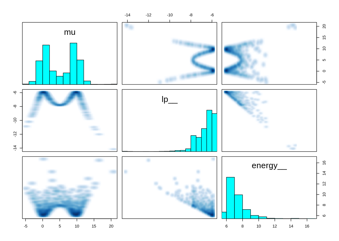
[1] 1000
[1] 1
[1] 1000
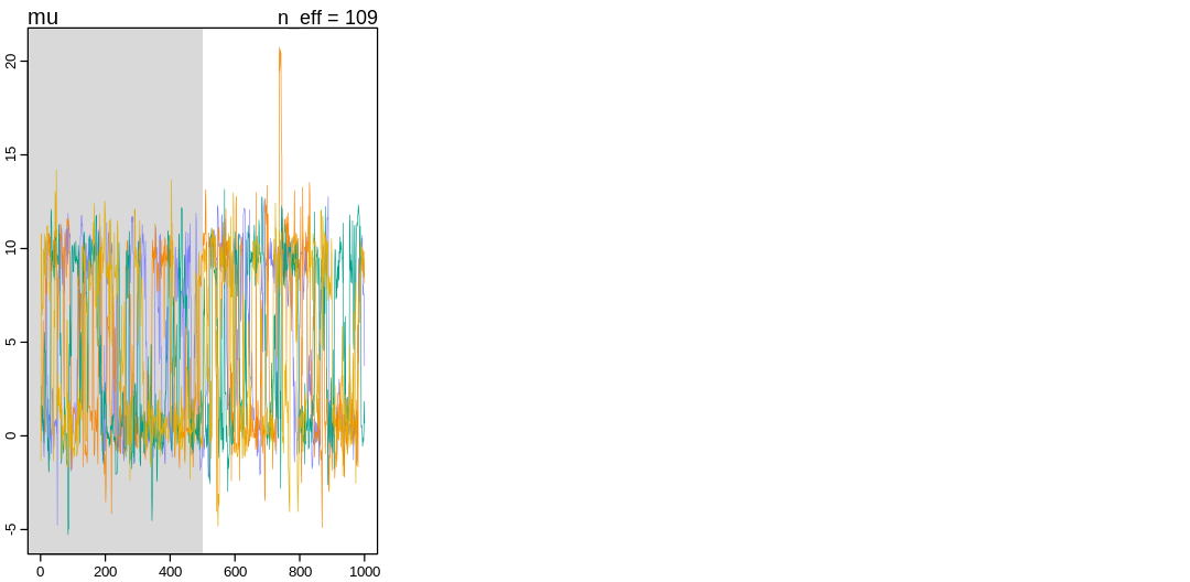
13H1. In 1980, a typical Bengali woman could have 5 or more children in her lifetime. By the
year 2000, a typical Bengali woman had only 2 or 3. You’re going to look at a historical set of
data, when contraception was widely available but many families chose not to use it. These data
reside in data(bangladesh) and come from the 1988 Bangladesh Fertility Survey. Each row is one of
1934 women. There are six variables, but you can focus on two of them for this practice problem:
district: ID number of administrative district each woman resided inuse.contraception: An indicator (0/1) of whether the woman was using contraception
The first thing to do is ensure that the cluster variable, district, is a contiguous set of
integers. Recall that these values will be index values inside the model. If there are gaps, you’ll
have parameters for which there is no data to inform them. Worse, the model probably won’t run. Look
at the unique values of the district variable:
R code 13.40
> sort(unique(d$district))

[1] 1 2 3 4 5 6 7 8 9 10 11 12 13 14 15 16 17 18 19 20 21 22 23 24 25
[26] 26 27 28 29 30 31 32 33 34 35 36 37 38 39 40 41 42 43 44 45 46 47 48 49 50
[51] 51 52 53 55 56 57 58 59 60 61
District 54 is absent. So district isn’t yet a good index variable, because it’s not contiguous.
This is easy to fix. Just make a new variable that is contiguous. This is enough to do it:
R code 13.41
> d$district_id <- as.integer(as.factor(d$district))
> sort(unique(d$district_id))

[1] 1 2 3 4 5 6 7 8 9 10 11 12 13 14 15 16 17 18 19 20 21 22 23 24 25
[26] 26 27 28 29 30 31 32 33 34 35 36 37 38 39 40 41 42 43 44 45 46 47 48 49 50
[51] 51 52 53 54 55 56 57 58 59 60
Now there are 60 values, contiguous integers 1 to 60. Now, focus on predicting use.contraception,
clustered by district_id. Fit both (1) a traditional fixed-effects model that uses an index
variable for district and (2) a multilevel model with varying intercepts for district. Plot the
predicted proportions of women in each district using contraception, for both the fixed-effects
model and the varying-effects model. That is, make a plot in which district ID is on the horizontal
axis and expected proportion using contraception is on the vertical. Make one plot for each model,
or layer them on the same plot, as you prefer. How do the models disagree? Can you explain the
pattern of disagreement? In particular, can you explain the most extreme cases of disagreement, both
why they happen where they do and why the models reach different inferences?
Answer. The help for the bangladesh data.frame, to confirm we aren’t missing anything:
data(bangladesh)
display(help(bangladesh))

bc_df <- bangladesh
bc_df$district_id <- as.integer(as.factor(bc_df$district))
sort(unique(bc_df$district_id))
| bangladesh {rethinking} | R Documentation |
Bangladesh contraceptive use data
Description
Contraceptive use data from 1934 Bangladeshi women.
Usage
data(bangladesh)
Format
woman : ID number for each woman in sample
district : Number for each district
use.contraception : 0/1 indicator of contraceptive use
living.children : Number of living children
age.centered : Centered age
urban : 0/1 indicator of urban context
References
Bangladesh Fertility Survey, 1989
- 1
- 2
- 3
- 4
- 5
- 6
- 7
- 8
- 9
- 10
- 11
- 12
- 13
- 14
- 15
- 16
- 17
- 18
- 19
- 20
- 21
- 22
- 23
- 24
- 25
- 26
- 27
- 28
- 29
- 30
- 31
- 32
- 33
- 34
- 35
- 36
- 37
- 38
- 39
- 40
- 41
- 42
- 43
- 44
- 45
- 46
- 47
- 48
- 49
- 50
- 51
- 52
- 53
- 54
- 55
- 56
- 57
- 58
- 59
- 60
The head of the bangladesh data.frame, with the new variable suggested by the author:
display(head(bc_df))
| woman | district | use.contraception | living.children | age.centered | urban | district_id | |
|---|---|---|---|---|---|---|---|
| <int> | <int> | <int> | <int> | <dbl> | <int> | <int> | |
| 1 | 1 | 1 | 0 | 4 | 18.4400 | 1 | 1 |
| 2 | 2 | 1 | 0 | 1 | -5.5599 | 1 | 1 |
| 3 | 3 | 1 | 0 | 3 | 1.4400 | 1 | 1 |
| 4 | 4 | 1 | 0 | 4 | 8.4400 | 1 | 1 |
| 5 | 5 | 1 | 0 | 1 | -13.5590 | 1 | 1 |
| 6 | 6 | 1 | 0 | 1 | -11.5600 | 1 | 1 |
A summary of the bangladesh data.frame:
display(summary(bc_df))
     woman           district     use.contraception living.children
 Min.   :   1.0   Min.   : 1.00   Min.   :0.0000    Min.   :1.000
 1st Qu.: 484.2   1st Qu.:14.00   1st Qu.:0.0000    1st Qu.:1.000
 Median : 967.5   Median :29.00   Median :0.0000    Median :3.000
 Mean   : 967.5   Mean   :29.35   Mean   :0.3925    Mean   :2.652
 3rd Qu.:1450.8   3rd Qu.:45.00   3rd Qu.:1.0000    3rd Qu.:4.000
 Max.   :1934.0   Max.   :61.00   Max.   :1.0000    Max.   :4.000
  age.centered            urban         district_id
 Min.   :-13.560000   Min.   :0.0000   Min.   : 1.00
 1st Qu.: -7.559900   1st Qu.:0.0000   1st Qu.:14.00
 Median : -1.559900   Median :0.0000   Median :29.00
 Mean   :  0.002198   Mean   :0.2906   Mean   :29.25
 3rd Qu.:  6.440000   3rd Qu.:1.0000   3rd Qu.:45.00
 Max.   : 19.440000   Max.   :1.0000   Max.   :60.00
Sampling from the fixed effects model:
bc_dat <- list(
  UseContraception = bc_df$use.contraception,
  DistrictId = bc_df$district_id
)

m_bc_fe <- ulam(
  alist(
    UseContraception ~ dbinom(1, p),
    logit(p) <- a[DistrictId],
    a[DistrictId] ~ dnorm(0, 1.5)
  ),
  data = bc_dat, chains = 4, cores = 4, log_lik = TRUE
)
display(precis(m_bc_fe, depth=2), mimetypes="text/plain")
iplot(function() {
  plot(precis(m_bc_fe, depth=2), main='m_bc_fe')
}, ar=0.8)
      mean          sd        5.5%       94.5%        n_eff    Rhat4
a[1]  -1.0547681689 0.2137850 -1.4113712 -0.717667817 4192.102 0.9986961
a[2]  -0.5855981344 0.4717542 -1.3520859  0.125955260 3223.185 0.9995662
a[3]   1.2550583484 1.1595008 -0.5349966  3.177147224 4249.073 0.9985745
a[4]   0.0052522427 0.3622941 -0.5692936  0.581238249 5704.123 0.9989137
a[5]  -0.5709354259 0.3285286 -1.0951361 -0.065205523 5477.596 0.9998667
a[6]  -0.8749469559 0.2580990 -1.3026629 -0.470909235 4472.230 0.9986760
a[7]  -0.9013248831 0.4971907 -1.7143530 -0.132134003 4350.855 0.9984769
a[8]  -0.4837459936 0.3371450 -1.0304723  0.063470078 4550.952 0.9990496
a[9]  -0.7869813762 0.4492103 -1.5267538 -0.090049801 4186.349 0.9996882
a[10] -1.9505405062 0.7253086 -3.2008269 -0.898679184 3471.160 0.9995382
a[11] -2.9533827816 0.8062259 -4.2617018 -1.796383362 4018.345 0.9989964
a[12] -0.6210314803 0.3654525 -1.2173021 -0.040618588 5205.563 0.9984615
a[13] -0.3282156478 0.4050214 -0.9691728  0.303809055 4008.268 0.9986197
a[14]  0.5115884255 0.1836011  0.2259073  0.810562013 5069.333 0.9995102
a[15] -0.5288315253 0.4306832 -1.2183537  0.156350803 3797.747 0.9985919
a[16]  0.1968089925 0.4434692 -0.4946812  0.934174012 4018.224 0.9991142
a[17] -0.8476844009 0.4400050 -1.5738591 -0.151441182 5606.310 0.9983207
a[18] -0.6513312317 0.3038974 -1.1215344 -0.188963354 3485.557 0.9983464
a[19] -0.4551743881 0.3897660 -1.0916403  0.180574052 5041.504 0.9991072
a[20] -0.3957950452 0.5056605 -1.2007204  0.386312996 3911.199 0.9988558
a[21] -0.4251602284 0.4539119 -1.1326079  0.285516031 4110.442 0.9996135
a[22] -1.2834923909 0.5199184 -2.1771181 -0.499955352 3721.947 1.0008591
a[23] -0.9352796145 0.5577795 -1.8839850 -0.081217902 4427.597 0.9986600
a[24] -2.0332675013 0.7332857 -3.2749123 -0.962836528 3762.332 0.9986260
a[25] -0.2063003707 0.2446207 -0.6033283  0.179821704 4516.826 0.9993179
a[26] -0.4317313211 0.5679176 -1.3411195  0.456665335 4186.062 0.9983912
a[27] -1.4433471879 0.3702887 -2.0342143 -0.866991965 3063.022 0.9993172
a[28] -1.0979455059 0.3270854 -1.6146927 -0.580667649 4831.533 0.9986556
a[29] -0.8966693304 0.4032127 -1.5428497 -0.271057874 4052.135 0.9989059
a[30] -0.0317843359 0.2520086 -0.4375573  0.369123314 5228.458 0.9991807
a[31] -0.1791887496 0.3575725 -0.7542883  0.408519554 5398.637 0.9987135
a[32] -1.2662656010 0.4627407 -2.0387609 -0.549057740 3897.366 0.9986331
a[33] -0.2747499521 0.4961998 -1.0755237  0.533220531 4436.955 0.9990616
a[34]  0.6303869056 0.3324131  0.1125598  1.163565844 3894.392 0.9988002
a[35]  0.0007613289 0.2880611 -0.4555591  0.444080649 4267.746 0.9991929
a[36] -0.5757697892 0.4987013 -1.3928939  0.196232261 4520.144 0.9987159
a[37]  0.1290149596 0.5530372 -0.7615294  1.011827794 5576.749 0.9985675
a[38] -0.8437549988 0.5501183 -1.7407113  0.005903183 5470.352 0.9983552
a[39]  0.0012694957 0.3912894 -0.6153342  0.622156787 4807.861 0.9985472
a[40] -0.1485404405 0.3220110 -0.6692041  0.348270907 4822.785 0.9993728
a[41] -0.0015475140 0.4001965 -0.6261782  0.645662040 5721.190 0.9986209
a[42]  0.1531121107 0.5529579 -0.7528373  1.062774192 3990.717 0.9991634
a[43]  0.1264317841 0.2996213 -0.3451562  0.584802894 4835.870 0.9991298
a[44] -1.2075757695 0.4509205 -1.9588258 -0.506909095 3295.934 0.9988037
a[45] -0.6765711108 0.3299037 -1.2096784 -0.146148167 4165.902 0.9987580
a[46]  0.0906947206 0.2169200 -0.2593299  0.436542049 3520.850 0.9984747
a[47] -0.1270971740 0.4941105 -0.9128387  0.632968795 4878.768 0.9993441
a[48]  0.0896217491 0.3021986 -0.3835983  0.568194371 4464.013 0.9990106
a[49] -1.7263563597 1.0271090 -3.5288819 -0.199839214 3669.684 0.9986273
a[50] -0.0980337730 0.4421999 -0.7889957  0.599278086 5419.794 0.9984798
a[51] -0.1570070979 0.3405839 -0.6962646  0.384063541 5156.160 0.9987228
a[52] -0.2281241353 0.2685612 -0.6726185  0.195834419 4232.174 0.9985204
a[53] -0.3036272976 0.4380177 -1.0075952  0.377601239 4089.384 0.9983238
a[54] -1.2217653559 0.8308343 -2.5974221  0.042572369 4092.345 0.9987841
a[55]  0.3093235995 0.2914719 -0.1561210  0.777189305 4355.213 0.9986629
a[56] -1.3914075160 0.4713755 -2.1549389 -0.665411585 2677.657 0.9993986
a[57] -0.1709203641 0.3370759 -0.7038543  0.357756114 3919.973 0.9989232
a[58] -1.7302958689 0.7613415 -3.0423049 -0.602380814 3831.756 0.9987976
a[59] -1.2147122087 0.4092811 -1.8780669 -0.574033077 3842.336 0.9992560
a[60] -1.2591466051 0.3508944 -1.8513903 -0.719459238 4456.370 0.9985475
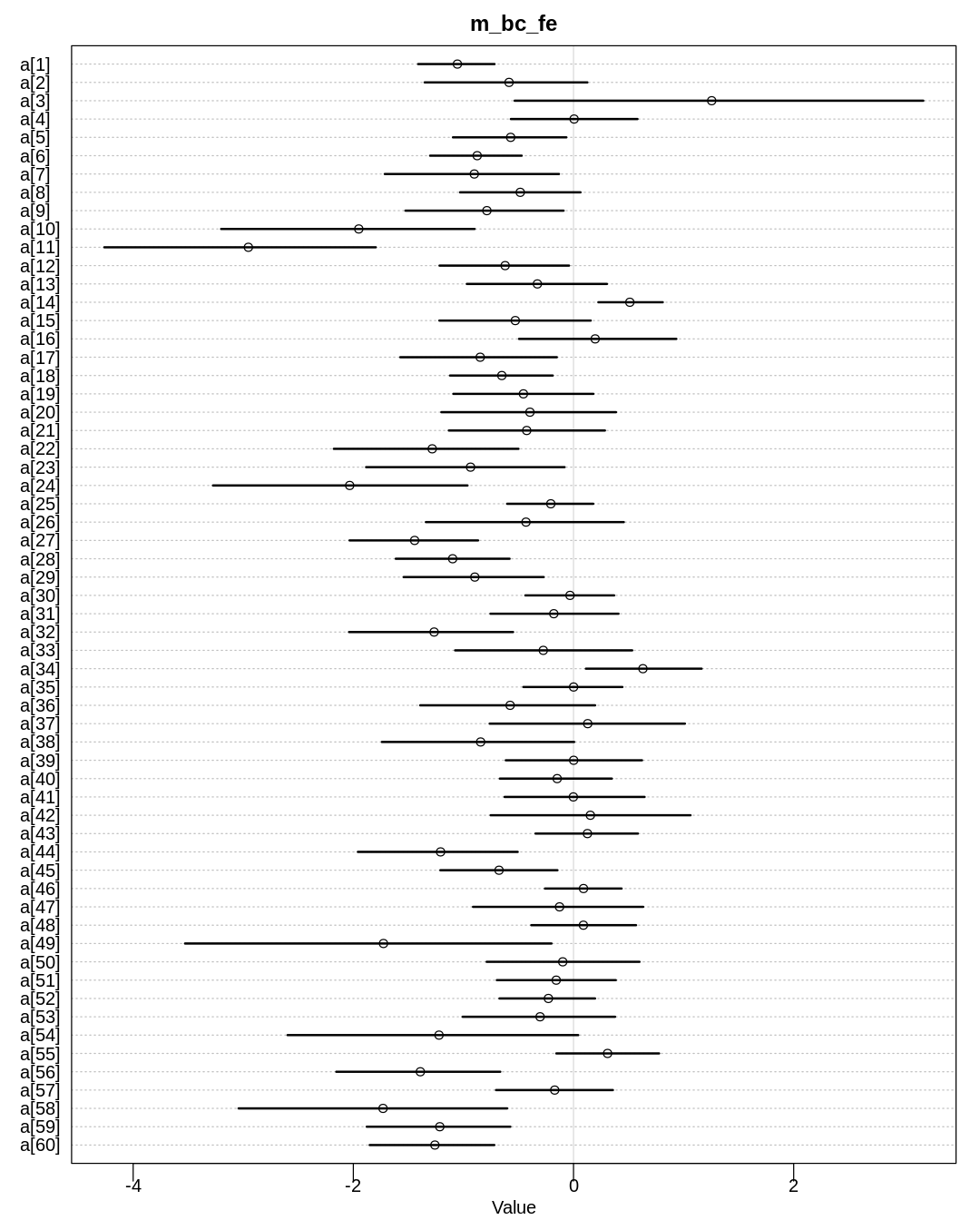
Sampling from the varying effects model:
m_bc_ve <- ulam(
  alist(
    UseContraception ~ dbinom(1, p),
    logit(p) <- a[DistrictId],
    a[DistrictId] ~ dnorm(a_bar, sigma),
    a_bar ~ dnorm(0, 1.5),
    sigma ~ dexp(1)
  ),
  data = bc_dat, chains = 4, cores = 4, log_lik = TRUE
)
display(precis(m_bc_ve, depth=2), mimetypes="text/plain")
iplot(function() {
  plot(precis(m_bc_ve, depth=2), main='m_bc_ve')
}, ar=0.8)

post_fe <- extract.samples(m_bc_fe)
post_ve <- extract.samples(m_bc_ve)
p_fe_c <- logistic(apply(post_fe$a, 2, mean))
p_ve_c <- logistic(apply(post_ve$a, 2, mean))
      mean         sd         5.5%       94.5%        n_eff     Rhat4
a[1]  -0.9911365   0.1874488  -1.2841565 -0.697323993 3724.069  0.9986166
a[2]  -0.5973283   0.3613326  -1.1887150 -0.038431148 3555.855  0.9988966
a[3]  -0.2534990   0.4932482  -1.0147419  0.540260179 2360.417  0.9989659
a[4]  -0.1897251   0.2869915  -0.6464395  0.272078861 3940.974  0.9993814
a[5]  -0.5631291   0.3025600  -1.0646529 -0.074426451 3624.225  0.9989869
a[6]  -0.8221548   0.2478595  -1.2324877 -0.438239250 2530.636  1.0003354
a[7]  -0.7547900   0.3680264  -1.3719530 -0.199882225 3268.395  1.0001832
a[8]  -0.5253510   0.2909768  -0.9968847 -0.070098722 4706.451  0.9993295
a[9]  -0.7047649   0.3490570  -1.2743097 -0.146081615 4097.080  0.9995121
a[10] -1.1371790   0.4275107  -1.8456066 -0.506439030 2463.665  0.9989101
a[11] -1.5375451   0.4368121  -2.2604115 -0.868793630 1829.279  1.0001064
a[12] -0.6069719   0.3137430  -1.1179321 -0.106477511 3773.145  0.9994154
a[13] -0.4114001   0.3216827  -0.9278973  0.095592442 4315.792  0.9990882
a[14]  0.3932803   0.1849226   0.1036812  0.698775124 2982.668  0.9999743
a[15] -0.5589397   0.3234493  -1.0862898 -0.066113505 4431.534  0.9993583
a[16] -0.1265695   0.3419858  -0.6723780  0.419188139 3336.782  0.9996718
a[17] -0.7405418   0.3396837  -1.2996079 -0.211062630 3859.886  0.9985521
a[18] -0.6338055   0.2591002  -1.0620451 -0.230075867 4195.865  0.9989785
a[19] -0.5070372   0.3299352  -1.0313660  0.009552186 3797.020  0.9983655
a[20] -0.4832641   0.3854034  -1.1299058  0.125409155 3169.711  1.0007198
a[21] -0.4879549   0.3385939  -1.0269999  0.061414762 2759.459  1.0012865
a[22] -0.9595981   0.3486549  -1.5324380 -0.416809417 3064.734  0.9986252
a[23] -0.7475987   0.3864535  -1.3670480 -0.142692472 3162.536  0.9997868
a[24] -1.1755111   0.4453223  -1.9342545 -0.504894376 2545.720  0.9984940
a[25] -0.2742567   0.2220537  -0.6224019  0.087584267 4007.146  0.9987441
a[26] -0.5118632   0.3762343  -1.1263524  0.078668075 2889.556  1.0004930
a[27] -1.1773818   0.3048968  -1.6911009 -0.697737886 2675.709  0.9986454
a[28] -0.9649865   0.2762108  -1.4220485 -0.532278438 3327.589  0.9992282
a[29] -0.7964959   0.3121289  -1.2936163 -0.303774115 3692.578  0.9984907
a[30] -0.1397838   0.2320535  -0.5186390  0.231159676 3268.204  0.9996337
⋮     ⋮            ⋮          ⋮          ⋮            ⋮         ⋮
a[33] -0.431074927 0.36078891 -1.0070316  0.13248620  3106.4879 0.9986770
a[34]  0.268804496 0.29313877 -0.1920465  0.76232467  2843.7107 0.9992301
a[35] -0.137373082 0.25346691 -0.5492551  0.27855563  3240.1599 0.9990327
a[36] -0.581503895 0.36028795 -1.1741271 -0.01349598  2987.4340 0.9994724
a[37] -0.222198678 0.36475878 -0.7974002  0.36254161  3493.3820 0.9995120
a[38] -0.712484784 0.38146158 -1.3219789 -0.11020644  3169.2858 0.9984891
a[39] -0.200399139 0.31415541 -0.6947224  0.29080620  3896.6873 0.9991367
a[40] -0.260503446 0.27873644 -0.7014452  0.18362604  4243.6551 0.9998715
a[41] -0.204316194 0.31525666 -0.7159777  0.29098687  3479.3094 0.9991047
a[42] -0.234861181 0.39769542 -0.9014570  0.38553967  2916.5487 0.9990804
a[43] -0.041829872 0.26291963 -0.4550113  0.37371403  3929.3624 0.9986894
a[44] -0.950316894 0.34405861 -1.5367159 -0.43130522  3174.0100 0.9984630
a[45] -0.657105765 0.28732486 -1.1253653 -0.20395486  3256.7921 0.9988105
a[46] -0.004683593 0.20140414 -0.3249970  0.31451062  2844.0269 0.9988385
a[47] -0.339132416 0.36201909 -0.9256789  0.23520108  4097.4534 0.9983989
a[48] -0.084488483 0.26776938 -0.5154784  0.34970546  4163.9774 0.9990185
a[49] -0.863038193 0.46947866 -1.6134919 -0.14994408  2502.9158 1.0006120
a[50] -0.297019559 0.33072976 -0.8254224  0.23944810  2784.5532 0.9994626
a[51] -0.270317309 0.26708038 -0.7004971  0.16030359  4151.5310 0.9992892
a[52] -0.293437787 0.22383035 -0.6455123  0.05050294  4242.8562 0.9988072
a[53] -0.426655424 0.35448550 -1.0019535  0.13610317  4584.2222 0.9990480
a[54] -0.784412276 0.46030201 -1.5210047 -0.07484807  4436.0743 0.9988564
a[55]  0.090184723 0.25630336 -0.3156922  0.49730657  3929.3675 1.0006963
a[56] -1.062681530 0.34762822 -1.6241983 -0.51756486  3111.5607 0.9993370
a[57] -0.300323347 0.29848730 -0.7686184  0.17260736  4306.2543 0.9988506
a[58] -1.010199303 0.44537117 -1.7124701 -0.32710344  3039.5226 0.9987960
a[59] -0.989726024 0.32189011 -1.5071225 -0.47070939  2563.2959 0.9989187
a[60] -1.043555423 0.29207770 -1.5446089 -0.57736213  3585.0769 0.9989461
a_bar -0.538589558 0.08555061 -0.6763500 -0.40304142  1913.3734 1.0012319
sigma  0.513375602 0.08172605  0.3946703  0.65255158   917.0302 1.0023959
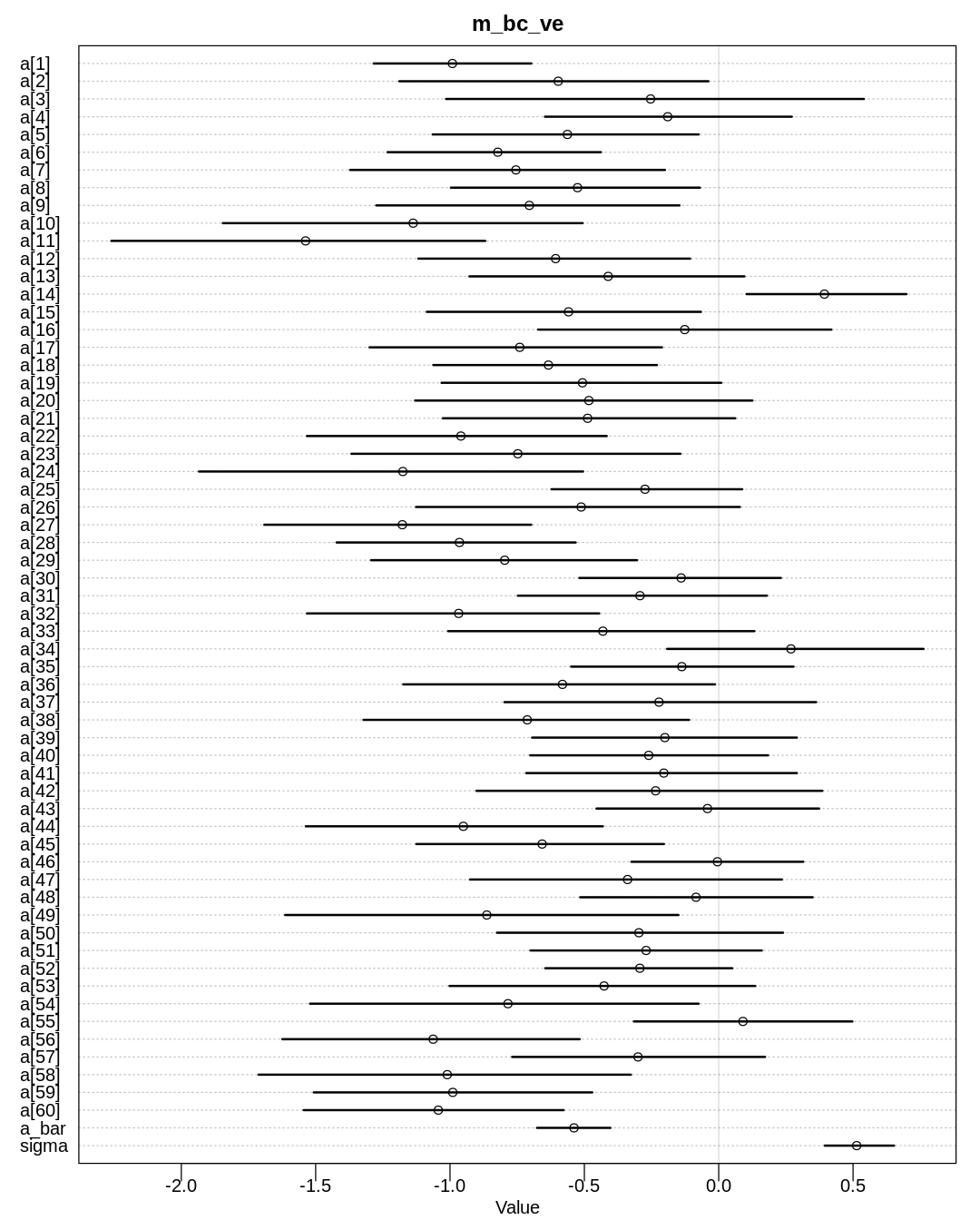
The plot suggested by the author in the question:
iplot(function() {
  plot(p_fe_c,
    ylim = c(0, 1), pch = 16, xaxt = "n",
    xlab = "district ID", ylab = "proportion using contraception", col = rangi2,
    main="Predicted proportion using contraception"
  )
  axis(1, at = seq(1, 60, by=2), las=2)

  # overlay posterior means
  points(p_ve_c)

  # mark posterior mean probability across districts
  abline(h = mean(inv_logit(post_ve$a_bar)), lty = 2)
})
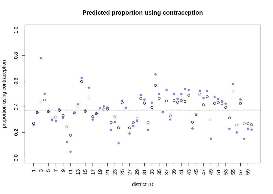
The number of observations (women) in every district:
iplot(function() {
  barplot(setNames(table(bc_df$district_id), sort(unique(bc_df$district_id))))
})
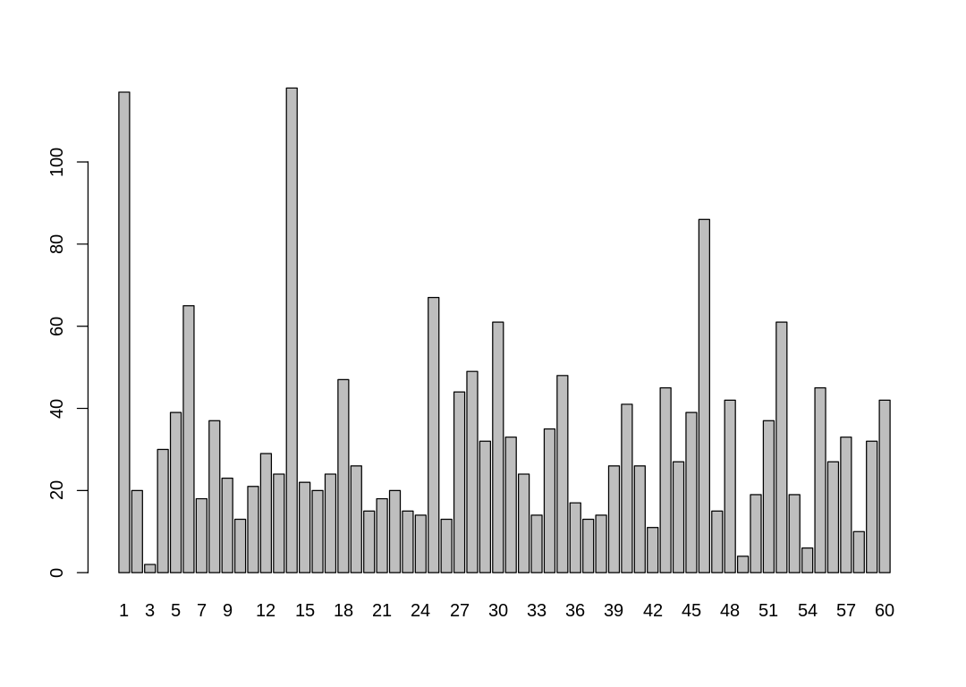
There are two factors affecting shrinkage, as discussed under Figure 13.1 in the text. The first is the number of observations in the district; notice that district 3 (with only a few observations) shrinks much more towards the weighted cluster mean (the dashed line) than any other district. The second is the distance from the dashed line. The estimate for district 35, which still has a reasonable number of observations, shrinks significantly towards the dashed line because it starts far from the mean. District 14 starts from a similar distance to the dashed line but shrinks less because it has so many observations.
13H2. Return to data(Trolley) from Chapter 12. Define and fit a varying intercepts model for
these data. Cluster intercepts on individual participants, as indicated by the unique values in the
id variable. Include action, intention, and contact as ordinary terms. Compare the varying
intercepts model and a model that ignores individuals, using both WAIC and posterior predictions.
What is the impact of individual variation in these data?
Answer. The head of the Trolley data.frame:
data(Trolley)
t_df <- Trolley
display(head(t_df))
| case | response | order | id | age | male | edu | action | intention | contact | story | action2 | |
|---|---|---|---|---|---|---|---|---|---|---|---|---|
| <fct> | <int> | <int> | <fct> | <int> | <int> | <fct> | <int> | <int> | <int> | <fct> | <int> | |
| 1 | cfaqu | 4 | 2 | 96;434 | 14 | 0 | Middle School | 0 | 0 | 1 | aqu | 1 |
| 2 | cfbur | 3 | 31 | 96;434 | 14 | 0 | Middle School | 0 | 0 | 1 | bur | 1 |
| 3 | cfrub | 4 | 16 | 96;434 | 14 | 0 | Middle School | 0 | 0 | 1 | rub | 1 |
| 4 | cibox | 3 | 32 | 96;434 | 14 | 0 | Middle School | 0 | 1 | 1 | box | 1 |
| 5 | cibur | 3 | 4 | 96;434 | 14 | 0 | Middle School | 0 | 1 | 1 | bur | 1 |
| 6 | cispe | 3 | 9 | 96;434 | 14 | 0 | Middle School | 0 | 1 | 1 | spe | 1 |
The help on the Trolley data.frame:
display(help(Trolley))
| Trolley {rethinking} | R Documentation |
Experimental data on ethical dilemmas
Description
These data comprise outcomes of experimental ethical dilemmas that are often called 'trolley' problems. Data kindly provided by Fiery Cushman.
Usage
data(Trolley)
Format
case: a code that combines treatment and story labels
response: participant's rating of appropriateness of action in story
order: integer order story appeared, within participant
id: participant id (factor)
age: participant's age in years
male: participant's gender; 1 for male, 0 for female
edu: participant's highest educational level
action: treatment code for story with action (1) or inaction (0)
intention: treatment code for intent (1) or lack of intent (0)
contact: treatmetn code for contact action (1) or lack of contact (0)
story: factor label for basic scenario modified by treatments
action2: alternative coding of action that is union of action and contact variables
References
Cushman et al. 2006. Psychological Science 17:1082–1089.
A summary of the Trolley data.frame:
display(summary(Trolley))
      case         response         order            id            age
 cfaqu  : 331   Min.   :1.000   Min.   : 1.0   96;434 :  30   Min.   :10.00
 cfbur  : 331   1st Qu.:3.000   1st Qu.: 9.0   96;445 :  30   1st Qu.:26.00
 cfrub  : 331   Median :4.000   Median :16.5   96;451 :  30   Median :36.00
 cibox  : 331   Mean   :4.199   Mean   :16.5   96;456 :  30   Mean   :37.49
 cibur  : 331   3rd Qu.:6.000   3rd Qu.:24.0   96;458 :  30   3rd Qu.:48.00
 cispe  : 331   Max.   :7.000   Max.   :32.0   96;466 :  30   Max.   :72.00
 (Other):7944                                  (Other):9750
      male                         edu           action         intention
 Min.   :0.000   Bachelor's Degree   :3540   Min.   :0.0000   Min.   :0.0000
 1st Qu.:0.000   Some College        :2460   1st Qu.:0.0000   1st Qu.:0.0000
 Median :1.000   Master's Degree     :1410   Median :0.0000   Median :0.0000
 Mean   :0.574   Graduate Degree     :1050   Mean   :0.4333   Mean   :0.4667
 3rd Qu.:1.000   High School Graduate: 870   3rd Qu.:1.0000   3rd Qu.:1.0000
 Max.   :1.000   Some High School    : 420   Max.   :1.0000   Max.   :1.0000
                 (Other)             : 180
    contact        story         action2
 Min.   :0.0   box    :1324   Min.   :0.0000
 1st Qu.:0.0   bur    :1324   1st Qu.:0.0000
 Median :0.0   spe    : 993   Median :1.0000
 Mean   :0.2   swi    : 993   Mean   :0.6333
 3rd Qu.:0.0   aqu    : 662   3rd Qu.:1.0000
 Max.   :1.0   boa    : 662   Max.   :1.0000
               (Other):3972
Let’s reproduce results for model m12.5 in the text:
t_dat <- list(
  R = t_df$response,
  A = t_df$action,
  I = t_df$intention,
  C = t_df$contact
)
m12.5 <- ulam(
  alist(
    R ~ dordlogit(phi, cutpoints),
    phi <- bA * A + bC * C + BI * I,
    BI <- bI + bIA * A + bIC * C,
    c(bA, bI, bC, bIA, bIC) ~ dnorm(0, 0.5),
    cutpoints ~ dnorm(0, 1.5)
  ),
  data = t_dat, chains = 4, cores = 4, log_lik = TRUE
)
display(precis(m12.5, depth = 2), mimetypes="text/plain")
iplot(function() {
  plot(precis(m12.5, depth=2), xlim=c(-6,8),main='m12.5')
}, ar=1.8)

plot_cutpoints <- function(model) {
  iplot(function() {
    par(mfrow=c(1,3))
    plot_intention <- function(kA, kC, model) {
      plot(NULL,
        type = "n", xlab = "intention", ylab = "probability",
        xlim = c(0, 1), ylim = c(0, 1), xaxp = c(0, 1, 1), yaxp = c(0, 1, 2),
        main=paste0("action=", kA, ", contact=", kC)
      )

      kI <- 0:1 # values of intention to calculate over
      pdat <- data.frame(A = kA, C = kC, I = kI, id=1)
      phi <- link(model, data = pdat)$phi

      post <- extract.samples(model)
      for (s in 1:50) {
        pk <- pordlogit(1:6, phi[s, ], post$cutpoints[s, ])
        for (i in 1:6) lines(kI, pk[, i], col = grau(0.1))
      }
    }
    plot_intention(0, 0, model)
    plot_intention(1, 0, model)
    plot_intention(0, 1, model)
  }, ar=2.2)
}

plot_hist <- function(model) {
  iplot(function() {
    par(mfrow=c(1,3))
    plot_intent <- function(kA, kC, model) {
        kI <- 0:1 # values of intention to calculate over
        pdat <- data.frame(A = kA, C = kC, I = kI, id=1)
        s <- sim(model, data = pdat)
        simplehist(s, xlab = "response", main=paste0("action=", kA, ", contact=", kC))
    }
    plot_intent(0, 0, model)
    plot_intent(1, 0, model)
    plot_intent(0, 1, model)
  }, ar=2.2)
}

plot_cutpoints(m12.5)
plot_hist(m12.5)
             mean       sd         5.5%       94.5%      n_eff     Rhat4
bIC          -1.2375932 0.09543187 -1.3890913 -1.0886818 1175.5217 1.001908
bIA          -0.4333412 0.07630972 -0.5513900 -0.3125365 1049.6312 1.005211
bC           -0.3425199 0.06711358 -0.4504975 -0.2386072 1140.6447 1.001802
bI           -0.2912295 0.05512958 -0.3813351 -0.2075464  805.5991 1.004812
bA           -0.4721490 0.05153728 -0.5522278 -0.3904029 1066.9576 1.003966
cutpoints[1] -2.6330227 0.05090999 -2.7158505 -2.5535491  935.4765 1.004076
cutpoints[2] -1.9380016 0.04728174 -2.0140466 -1.8620192  930.2425 1.003504
cutpoints[3] -1.3437476 0.04524626 -1.4155249 -1.2698631  877.9480 1.002820
cutpoints[4] -0.3083380 0.04284013 -0.3767162 -0.2396050  992.4171 1.001940
cutpoints[5]  0.3617297 0.04292332  0.2942512  0.4311708 1034.7950 1.001985
cutpoints[6]  1.2672309 0.04527226  1.1964799  1.3390448 1343.7071 1.001424
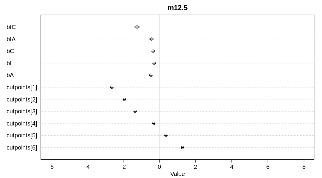
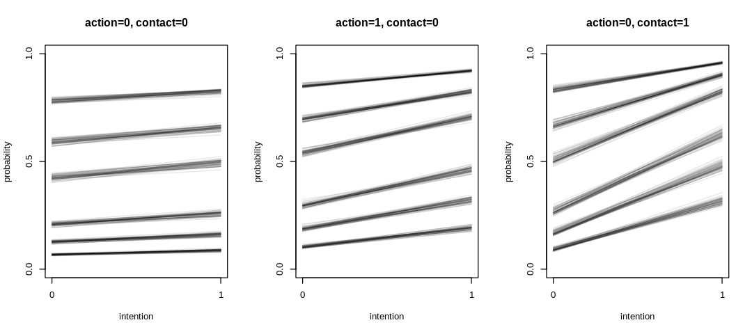
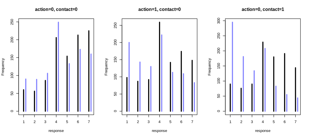
We’ll use the following model with id clusters:
Notice we do not provide a cluster mean \(\bar{\alpha}\); this variable would be non-identifiable with respect to the intercepts in the ordered logit. If you try to add this parameter, you’ll see the divergent transitions and poor sampling characteristic of this problem.
Sampling from the model with id clusters:
t_id_dat <- list(
  R = t_df$response,
  A = t_df$action,
  I = t_df$intention,
  id = t_df$id,
  C = t_df$contact
)
m_trolley_id <- ulam(
  alist(
    R ~ dordlogit(phi, cutpoints),
    phi <- a[id] + bA * A + bC * C + BI * I,
    a[id] ~ dnorm(0, sigma),
    sigma ~ dexp(1),
    BI <- bI + bIA * A + bIC * C,
    c(bA, bI, bC, bIA, bIC) ~ dnorm(0, 0.5),
    cutpoints ~ dnorm(0, 1.5)
  ),
  data = t_id_dat, chains = 4, cores = 4, log_lik = TRUE, iter=800
)
display(precis(m_trolley_id, depth = 2), mimetypes="text/plain")
Warning message:
“Bulk Effective Samples Size (ESS) is too low, indicating posterior means and medians may be unreliable.
Running the chains for more iterations may help. See
https://mc-stan.org/misc/warnings.html#bulk-ess”
Warning message:
“Tail Effective Samples Size (ESS) is too low, indicating posterior variances and tail quantiles may be unreliable.
Running the chains for more iterations may help. See
https://mc-stan.org/misc/warnings.html#tail-ess”
             mean        sd         5.5%        94.5%       n_eff     Rhat4
a[1]         -0.56353317 0.2961871  -1.02180217 -0.09805443  609.4124 1.0005135
a[2]         -1.75769877 0.4366643  -2.46081067 -1.05799696 1374.2609 0.9985736
a[3]         -2.96541068 0.4173908  -3.64774547 -2.31760922 1070.1699 0.9996611
a[4]         -0.37053427 0.4761909  -1.13348728  0.38172148 1209.9746 1.0002442
a[5]         -3.46992394 0.4332231  -4.18261279 -2.80619157 1249.0739 1.0031403
a[6]          0.63332401 0.3174243   0.11606255  1.12686623  750.1932 1.0022227
a[7]         -0.46657182 0.3209316  -0.98671807  0.04852067  721.1306 1.0034259
a[8]          3.85997536 0.4975133   3.09604198  4.67143047 1294.1944 1.0013937
a[9]         -0.87006827 0.3199011  -1.37586817 -0.35114960  589.8566 1.0041920
a[10]         0.77257066 0.3344652   0.21815818  1.28903980  698.9720 1.0080996
a[11]         0.58163790 0.3429877   0.03486364  1.13120264  712.7327 1.0014701
a[12]         2.39164951 0.3897521   1.77621261  3.02176079  973.2805 0.9997558
a[13]        -0.43860210 0.3162860  -0.94455169  0.06649594  633.6931 1.0014437
a[14]        -1.00885293 0.3423811  -1.55262975 -0.46208981  792.1098 1.0029308
a[15]         1.62317172 0.3196033   1.13065485  2.13118339  655.2993 1.0018768
a[16]        -1.85514675 0.4180702  -2.50067525 -1.17784524 1363.9095 1.0039794
a[17]         1.59304146 0.4451567   0.87763670  2.27107819 1204.9260 0.9998765
a[18]        -1.21473989 0.3588845  -1.78193099 -0.65530368  875.4417 1.0012111
a[19]        -1.32521070 0.3157718  -1.86585500 -0.83017463  866.0450 1.0010094
a[20]        -0.52783541 0.2999337  -0.98511706 -0.03742998  528.3042 1.0042488
a[21]        -2.14824735 0.3402819  -2.70621545 -1.59529493  739.2898 1.0023227
a[22]        -0.02678743 0.3661637  -0.60340204  0.56346466  779.7531 1.0015685
a[23]        -5.23144825 0.6241298  -6.32654285 -4.31990665 1223.4801 1.0023636
a[24]        -1.67222594 0.3099048  -2.17495014 -1.17642989  704.4844 1.0031817
a[25]        -0.68463486 0.3240165  -1.20124259 -0.17489539  835.4960 1.0002229
a[26]         0.92698878 0.3511169   0.35895447  1.49579364  949.6574 1.0017567
a[27]         1.09466960 0.4395155   0.39502070  1.78836931 1348.9841 1.0014579
a[28]        -0.82685263 0.3581814  -1.40157906 -0.24647796  960.6689 1.0035368
a[29]         1.17488007 0.3290987   0.65462994  1.71830911  668.6289 1.0037767
a[30]         1.65701666 0.3492145   1.10556087  2.24158374  894.4211 1.0036917
⋮            ⋮           ⋮          ⋮           ⋮           ⋮         ⋮
a[314]       -1.3542568  0.32945432 -1.86742764 -0.82142138  971.6676 1.0020511
a[315]       -0.8540011  0.34241482 -1.39386953 -0.31436297  624.9605 1.0050265
a[316]        1.4812958  0.32448888  0.93933320  1.99329093  638.4552 1.0002180
a[317]       -0.8066667  0.33949087 -1.37586028 -0.29679957  671.0560 1.0043909
a[318]       -0.8339491  0.32464892 -1.35563812 -0.29373991  689.0683 1.0020395
a[319]       -0.3601915  0.29239934 -0.82979913  0.12130636  714.9171 1.0039653
a[320]       -1.7844106  0.36109067 -2.34479272 -1.20211265  946.4787 1.0025796
a[321]       -1.7523853  0.35275445 -2.30124278 -1.19702351  724.7850 1.0038180
a[322]        4.0188856  0.44091784  3.33944830  4.75967169  970.0613 1.0018672
a[323]        0.2192927  0.33185887 -0.30365605  0.74333970  753.3259 1.0048503
a[324]        6.1394695  0.80943044  4.96839059  7.50448881 1970.4292 0.9983066
a[325]       -1.2142048  0.58523731 -2.13481130 -0.28469151 1863.5302 0.9986617
a[326]        0.6195830  0.33119313  0.09059312  1.13023415  684.4746 0.9996006
a[327]       -0.3058018  0.32691683 -0.81558409  0.21422232  804.3834 1.0021583
a[328]        1.7048587  0.33147722  1.17414277  2.22621687  741.0444 1.0012876
a[329]       -1.2521281  0.32081154 -1.74845916 -0.74499073  585.1115 1.0066785
a[330]       -3.4222229  0.42437841 -4.13034469 -2.74412580  844.9541 1.0041652
a[331]       -0.5978400  0.38576024 -1.22200816  0.03604231  917.3723 1.0020468
sigma         1.9143741  0.07695070  1.79496507  2.04170111 1877.4210 0.9996872
bIC          -1.6686659  0.10200631 -1.83669982 -1.51108365 1004.1502 1.0000917
bIA          -0.5591247  0.08465414 -0.69482550 -0.42699295  990.1649 1.0005712
bC           -0.4516718  0.07158114 -0.56303007 -0.33464898  905.3852 1.0001007
bI           -0.3851002  0.06230474 -0.48105230 -0.28248089  788.8813 0.9994695
bA           -0.6486070  0.05739569 -0.73743063 -0.55605901 1017.0408 0.9987082
cutpoints[1] -3.7188728  0.11839125 -3.91090361 -3.52899919  114.0915 1.0308318
cutpoints[2] -2.7694481  0.11584907 -2.95671145 -2.58437139  109.0320 1.0339041
cutpoints[3] -1.9653730  0.11524119 -2.15138635 -1.78470696  107.3575 1.0335104
cutpoints[4] -0.4676383  0.11422623 -0.65270587 -0.28169906  105.5194 1.0337652
cutpoints[5]  0.5818210  0.11573294  0.39648815  0.76722987  107.4401 1.0316479
cutpoints[6]  1.9903550  0.11933490  1.79906822  2.18108821  113.1717 1.0306061
Although it may seem excessive, here are all the id parameter estimates on the same x-axis scale
as the precis plot above for model m12.5:
iplot(function() {
  plot(precis(m_trolley_id, depth=2), xlim=c(-6,8), main='m_trolley_id')
}, ar=0.2)
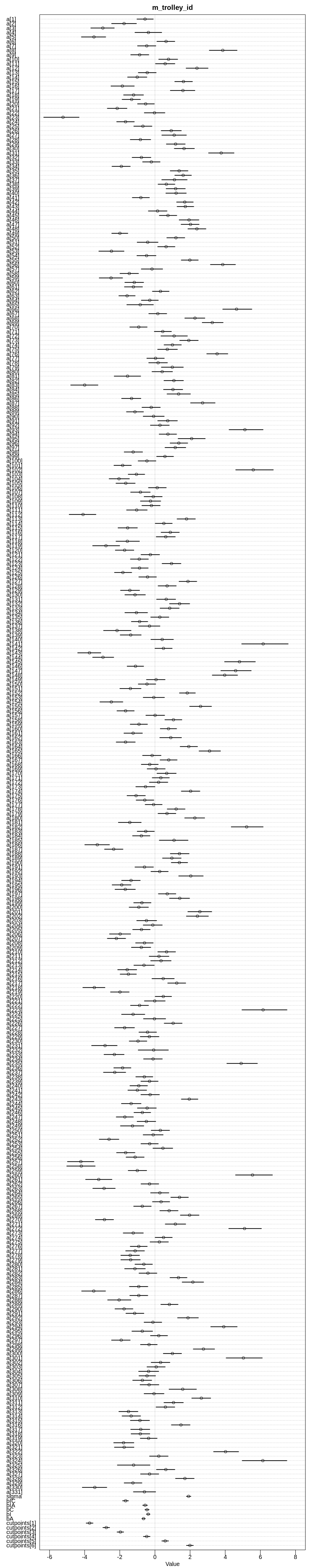
Notice the individual intercepts are much less certain than sigma, bIC, and the other
higher-level parameters. This uncertainty leads to the more variable posterior predictive plot in
the first triptych below. These two tripytch plots for a typical individual, specifically the
individual with id equal 1, who did not have a strong positive or negative tendency.
plot_cutpoints(m_trolley_id)
plot_hist(m_trolley_id)

display_markdown("
Comparing the models using WAIC:
")
iplot(function() {
  plot(compare(m12.5, m_trolley_id))
}, ar=4.5)

display_markdown("
Comparing the models using PSIS, to check for overfitting or outliers:
")
iplot(function() {
  plot(compare(m12.5, m_trolley_id, func=PSIS))
}, ar=4.5)
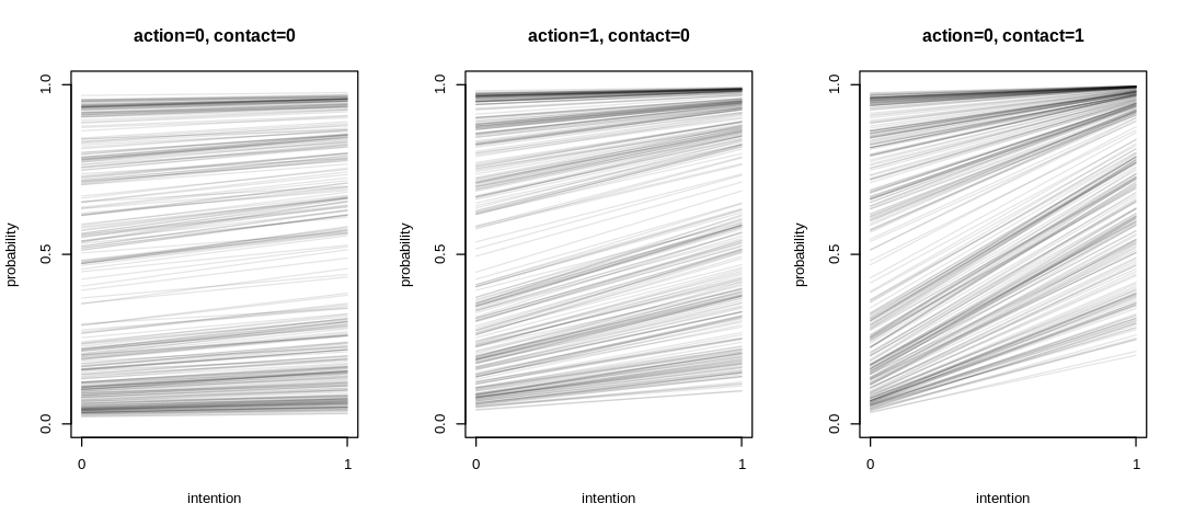
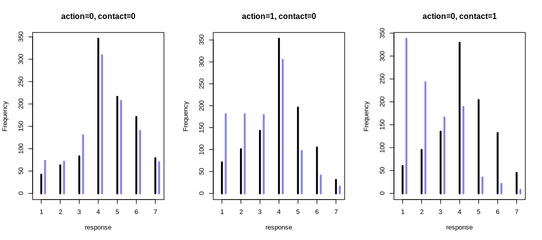
Comparing the models using WAIC:
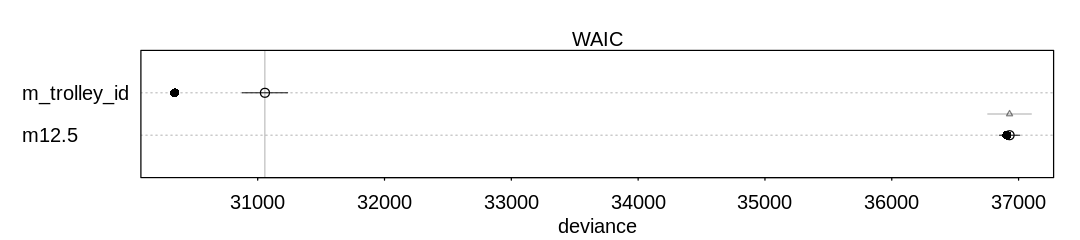
Comparing the models using PSIS, to check for overfitting or outliers:
Some Pareto k values are high (>0.5). Set pointwise=TRUE to inspect individual points.
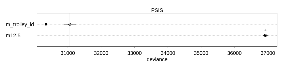
The new model has a much lower WAIC/PSIS score because the new predictor explains much of the
unexplained variation in the previous model (notice the large inferred mean for sigma).
13H3. The Trolley data are also clustered by story, which indicates a unique narrative for
each vignette. Define and fit a cross-classified varying intercepts model with both id and
story. Use the same ordinary terms as in the previous problem. Compare this model to the previous
models. What do you infer about the impact of different stories on responses?
Answer. Sampling from the suggested model:
data(Trolley)
t_df <- Trolley

t_story_id_dat <- list(
  R = t_df$response,
  A = t_df$action,
  I = t_df$intention,
  id = t_df$id,
  story = as.integer(t_df$story),
  C = t_df$contact
)
m_trolley_story_id <- ulam(
  alist(
    R ~ dordlogit(phi, cutpoints),
    phi <- a[id] + b[story] + bA * A + bC * C + BI * I,
    a[id] ~ dnorm(0, sigma_a),
    sigma_a ~ dexp(1),
    b[story] ~ dnorm(0, sigma_b),
    sigma_b ~ dexp(1),
    BI <- bI + bIA * A + bIC * C,
    c(bA, bI, bC, bIA, bIC) ~ dnorm(0, 0.5),
    cutpoints ~ dnorm(0, 1.5)
  ),
  data = t_story_id_dat, chains = 4, cores = 4, log_lik = TRUE, iter=800
)
display(precis(m_trolley_story_id, depth = 2), mimetypes="text/plain")
iplot(function() {
  plot(precis(m_trolley_story_id, depth=2), xlim=c(-6,8), main='m_trolley_story_id')
}, ar=0.18)
Warning message:
“The largest R-hat is 1.06, indicating chains have not mixed.
Running the chains for more iterations may help. See
https://mc-stan.org/misc/warnings.html#r-hat”
Warning message:
“Bulk Effective Samples Size (ESS) is too low, indicating posterior means and medians may be unreliable.
Running the chains for more iterations may help. See
https://mc-stan.org/misc/warnings.html#bulk-ess”
Warning message:
“Tail Effective Samples Size (ESS) is too low, indicating posterior variances and tail quantiles may be unreliable.
Running the chains for more iterations may help. See
https://mc-stan.org/misc/warnings.html#tail-ess”
             mean        sd         5.5%        94.5%       n_eff
a[1]         -0.56316487 0.3062317  -1.04866012 -0.08303912  700.1520
a[2]         -1.70264993 0.4463165  -2.38798429 -0.95805328 1269.7956
a[3]         -3.03816922 0.4212535  -3.70576458 -2.36267427 1221.3509
a[4]         -0.39840814 0.4607174  -1.11824362  0.33492908 1987.7908
a[5]         -3.53627392 0.4212684  -4.25853409 -2.90347294 1112.0019
a[6]          0.67017225 0.3182554   0.17001121  1.18672970  670.9657
a[7]         -0.40558820 0.3197392  -0.91008963  0.11270959  704.1311
a[8]          3.95010049 0.4669430   3.24021992  4.73336448 1299.1907
a[9]         -0.87778821 0.3126278  -1.36629041 -0.37457437  636.1947
a[10]         0.79689158 0.3387809   0.26862455  1.35358976  905.3176
a[11]         0.56853755 0.3567595   0.02087721  1.12585481  910.6981
a[12]         2.43042937 0.3657701   1.84698263  3.00068292 1295.9689
a[13]        -0.44351859 0.3020161  -0.92608546  0.05152353  646.9133
a[14]        -0.99103075 0.3281953  -1.51986956 -0.47570117  672.2905
a[15]         1.72993150 0.3317421   1.19972529  2.26167304  646.7812
a[16]        -1.89165803 0.4215558  -2.55985563 -1.23807219 1494.2323
a[17]         1.67720096 0.4735600   0.89432934  2.42044364 1336.5860
a[18]        -1.17242059 0.3467013  -1.73047967 -0.61884137 1096.5816
a[19]        -1.36327308 0.3156245  -1.85102495 -0.86337880  668.7573
a[20]        -0.53714499 0.2937734  -1.01418880 -0.06291586  795.5939
a[21]        -2.18408098 0.3561207  -2.74291209 -1.58525155  573.6218
a[22]         0.01515743 0.3743190  -0.60486391  0.60575978  827.9334
a[23]        -5.38259002 0.5928650  -6.35802119 -4.47518875 2352.7562
a[24]        -1.74776990 0.3155132  -2.24725506 -1.22288890  789.6467
a[25]        -0.67922782 0.3345888  -1.21942041 -0.15029700  677.7735
a[26]         0.91663072 0.3129825   0.42169584  1.40920127  719.7911
a[27]         1.08895725 0.4545951   0.35963490  1.80504876 1621.3281
a[28]        -0.82124038 0.3653313  -1.39906499 -0.21555552  826.5497
a[29]         1.23325809 0.3270985   0.70574788  1.74797048 1281.7369
a[30]         1.73635245 0.3296675   1.18662216  2.26371802  730.6892
⋮            ⋮           ⋮          ⋮           ⋮           ⋮
a[327]       -0.28662965 0.32968612 -0.8397690   0.22969090  889.14997
a[328]        1.73420600 0.32667940  1.2170105   2.26672644 1052.55393
a[329]       -1.29204269 0.31889777 -1.8001379  -0.77876378  782.93440
a[330]       -3.53235839 0.46302658 -4.2753005  -2.82080683 1239.20399
a[331]       -0.59046808 0.37514898 -1.1714589   0.01492163  850.98552
sigma_a       1.96610510 0.08467663  1.8350399   2.10567674 3118.02782
b[1]          0.92967879 0.19845686  0.6396093   1.25019007  106.70089
b[2]         -0.07238916 0.19505092 -0.3564759   0.24083207   86.66171
b[3]          0.08209595 0.18364279 -0.1724035   0.37996989   92.58106
b[4]          0.62321817 0.19218158  0.3449638   0.94013540   94.68768
b[5]          0.03032877 0.18893382 -0.2369821   0.32915908   98.89361
b[6]          0.12069973 0.18969155 -0.1478143   0.43278542  112.35333
b[7]         -0.56876205 0.18869525 -0.8392746  -0.25774645  114.70110
b[8]          0.03602667 0.19545684 -0.2488369   0.35041177  115.67326
b[9]         -0.37852292 0.19095179 -0.6585248  -0.06312420   91.39244
b[10]         0.87280587 0.19511909  0.5830461   1.19022737   90.69660
b[11]        -0.27013388 0.18930543 -0.5473264   0.02937101   99.04665
b[12]        -0.24966498 0.18685623 -0.5181914   0.05921666   94.23037
sigma_b       0.54517184 0.14154137  0.3711658   0.80338096  299.61242
bIC          -1.28787914 0.11266707 -1.4702146  -1.11203088 1201.87531
bIA          -0.52890152 0.08192155 -0.6623173  -0.39963644 1372.01715
bC           -1.07536950 0.09578888 -1.2261345  -0.92467002 1154.81943
bI           -0.45759246 0.06766379 -0.5673367  -0.34981692 1113.66532
bA           -0.89126583 0.06763231 -1.0002158  -0.78328436 1112.15073
cutpoints[1] -3.91752790 0.21080380 -4.2384182  -3.56319039   83.33309
cutpoints[2] -2.94166839 0.20888383 -3.2618960  -2.59017921   81.56924
cutpoints[3] -2.11014952 0.20704331 -2.4246454  -1.76567932   82.26298
cutpoints[4] -0.56232537 0.20579724 -0.8680882  -0.21451455   81.88016
cutpoints[5]  0.51961396 0.20579640  0.2155380   0.85862691   83.20928
cutpoints[6]  1.96266241 0.20728119  1.6549095   2.31161821   84.86356
             Rhat4
a[1]         1.0043664
a[2]         1.0026881
a[3]         1.0023259
a[4]         0.9991884
a[5]         1.0019290
a[6]         1.0046831
a[7]         1.0035200
a[8]         1.0019186
a[9]         1.0072141
a[10]        1.0045010
a[11]        1.0017051
a[12]        1.0007463
a[13]        1.0035501
a[14]        1.0052138
a[15]        1.0046899
a[16]        1.0016086
a[17]        1.0015974
a[18]        1.0020826
a[19]        1.0041743
a[20]        1.0021651
a[21]        1.0090934
a[22]        1.0040289
a[23]        1.0005327
a[24]        1.0036648
a[25]        1.0011532
a[26]        1.0044393
a[27]        0.9998108
a[28]        1.0036460
a[29]        1.0005073
a[30]        1.0052238
⋮            ⋮
a[327]       1.0016571
a[328]       1.0009393
a[329]       1.0040270
a[330]       1.0010456
a[331]       1.0061746
sigma_a      0.9989950
b[1]         1.0591266
b[2]         1.0681644
b[3]         1.0614984
b[4]         1.0674420
b[5]         1.0564720
b[6]         1.0560444
b[7]         1.0555663
b[8]         1.0550387
b[9]         1.0578995
b[10]        1.0612750
b[11]        1.0631018
b[12]        1.0590566
sigma_b      1.0269283
bIC          0.9989761
bIA          0.9993492
bC           0.9991989
bI           0.9992121
bA           1.0001422
cutpoints[1] 1.0460215
cutpoints[2] 1.0463412
cutpoints[3] 1.0462888
cutpoints[4] 1.0463179
cutpoints[5] 1.0458839
cutpoints[6] 1.0448288
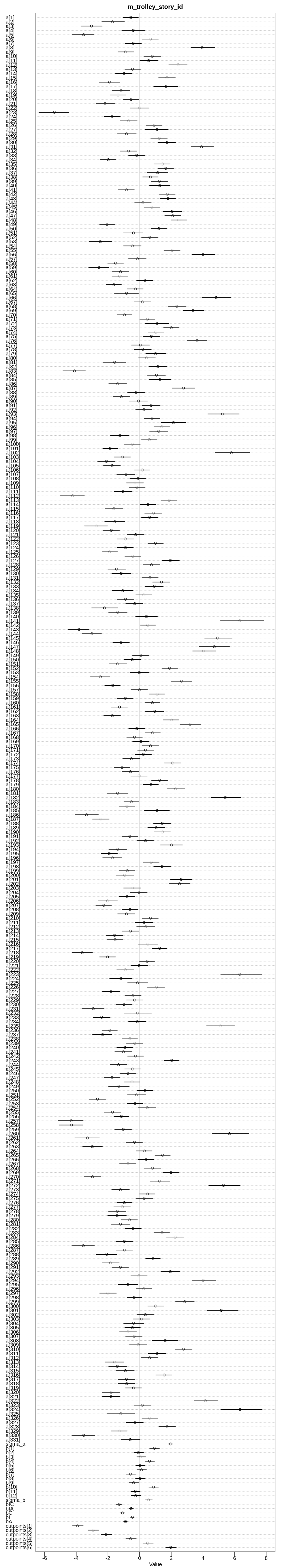
Comparing the models using WAIC:
iplot(function() {
  plot(compare(m12.5, m_trolley_id, m_trolley_story_id))
}, ar=4.5)

Comparing the models using PSIS, to check for overfitting or outliers:
iplot(function() {
  plot(compare(m12.5, m_trolley_id, m_trolley_story_id, func=PSIS))
}, ar=4.5)
Some Pareto k values are high (>0.5). Set pointwise=TRUE to inspect individual points.
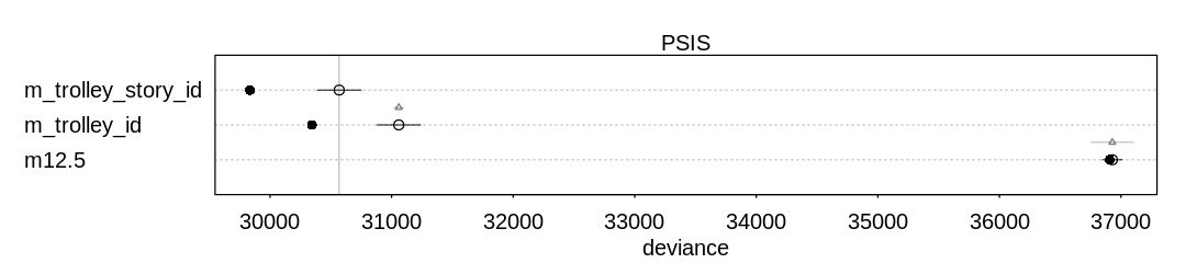
With this new predictor, our inferences about bIC, bA and similar parameters have changed
more significantly. Presumably these individual stories provide even more detail than the contact,
action, etc. indicators and are potentially redundant or non-identifiable with respect to the
parameters attached to the indicator variables.
Still, this extra detail seems to provide significant predictive power according to WAIC and PSIS, though not to the same degree that the individual variable helped prediction.