3.3. Functors, natural transformations#
3.3.1 Sets and functions as databases#
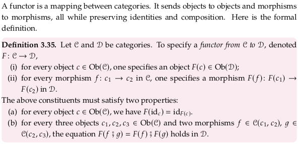
3.3.2 Functors#
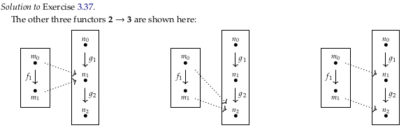
Exercise 3.37#

A fourth functor sends \(F(m_0) = n_1\), \(F(f_1) = n_1\), and \(F(m_1) = n_1\) (that is, it sends everything to \(n_1\)). A fifth functor sends everything to \(n_2\). A sixth sends \(F(m_0) = n_1\), \(F(f_1) = g_2\), and \(F(m_1) = n_2\).
Reveal 7S answer
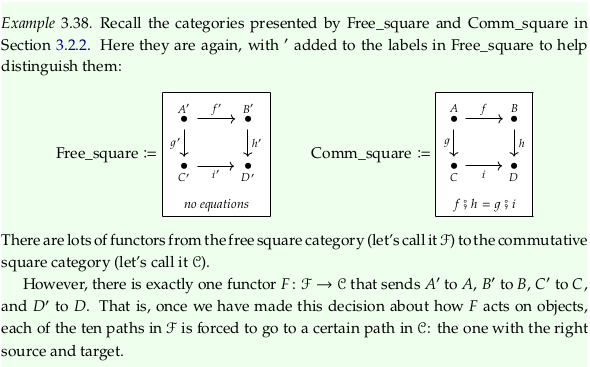
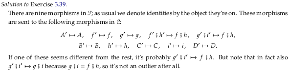
Exercise 3.39#

A’ is sent to A, f’ to f, B’ to B, g’ to g, h’ to h, C’ to C, i’ to i, and D’ to D (covering eight of the morphisms). The morphisms g’;i’ and f’;h’ are both sent to f;h = g;i.
Reveal 7S answer
Exercise 3.40#
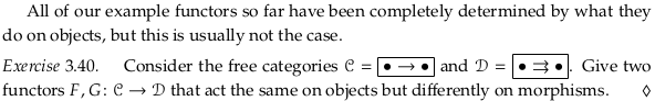
The only arrow in C (call it f) could be sent to either arrow in D (call them g and h). You can’t send f to both g and h because a functor only returns one morphism (like a function).
Said another way, you can’t draw blue lines as in Example 3.36 between these two categories as a “sufficient” answer (it doesn’t fully specify a functor).
Reveal 7S answer
The author’s answer seems confused; he asks for two functors in the question and gives four in the answer.
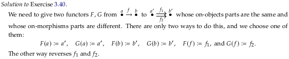
Example 3.42#
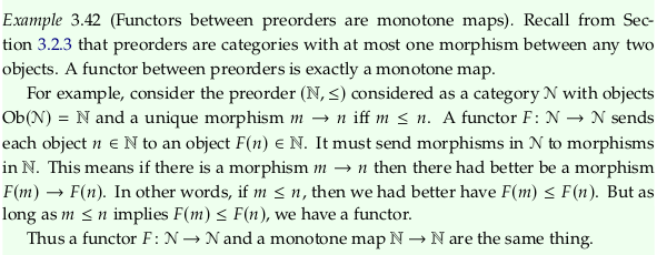
See the errata. I’d go one step beyond the errata and rephrase this example as the following:

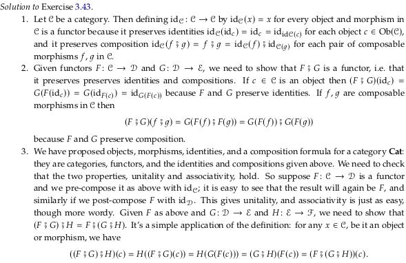
Exercise 3.43#
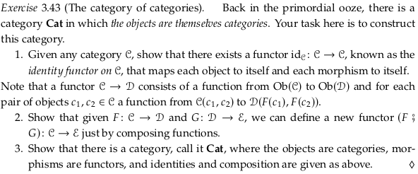
Prerequisite to Category of small categories.
For 1., it’s trivial to check the two properties required of a functor (preserving identities and
composition). The property (a) is satisfied by definition of sending every object (category) to
itself i.e. that \(F(id_c) = id_c = id_{F(c)_{}}\). For property (b) we clearly have \(F(f ⨾ g) = F(f)
⨾ F(g)\) because \(F(f) = f\) and \(F(g) = g\) and \(F(f ⨾ g) = f ⨾ g\). Call this \(id_{𝓒_{}} = F\).
For 2., we must first construct this second new functor \(H\) where morphisms are functors. Use the
subscript \(Ob\) to refer to the part of a functor that deals with mapping objects (categories). To
satisfy (i) in our definition of a functor, we construct the function \(H_{Ob_{}} : Ob(C)\) → \(Ob(E)\)
by simply composing the two functions \(F_{Ob_{}} : Ob(C)\) → \(Ob(D)\) and \(G_{Ob_{}} : Ob(D)\) →
\(Ob(E)\). That is, \(H_{Ob_{}} = F_{Ob_{}} ⨾ G_{Ob_{}}\).
To satisfy (ii), use the subscript \(m\) to refer to the part of a functor that deals with mapping morphisms (here, functors) between objects (categories). Our construction will simply compose the two functions \(F_m : C(c_1,c_2) → D(F(c_1),F(c_2))\) and \(G_m : D(d_1,d_2)\) → \(E(G(d_1),G(d_2))\). That is, \(H_m = F_m ⨾ G_m\).
Now we must check this construction \(H\) preserves identities and composition. To show it preserves identities we must show that for every object \(c \in Ob(C)\) we have \(H(id_c) = F⨾G(id_c) = id_{F⨾G(c)_{}}\). Because \(F\) and \(G\) are both functors, we have that \(F(id_c) = id_{F(c)_{}}\) (similarly for \(G\)) so that \(F⨾G(id_c) = id_{F(c)_{}}⨾G = id_{G(F(c))_{}}\), which is equivalent to what we wanted to show.
To show it preserves composition, we must show that for every morphism \(f\) and \(g\) in Cat where the target of \(f\) is the source of \(g\) that \(F⨾G(f⨾g) = F⨾G(f)⨾F⨾G(g)\). Because F and G are functors we have \(F⨾G(f⨾g) = F(f)⨾F(g);G = G(F(f)⨾F(g)) = G(F(f))⨾G(F(g))\). To summarize, because \(F\) and \(G\) preserve identities and composition then \(H\) does as well.
For 3., we need to satisfy all the conditions in Definition 3.6. For (i), we are specifying a
collection of objects that is all categories. For (ii), for every two objects c,d the set C(c,d)
will be the set of all functors from the categories c and d. For (iii), we can use the identity
functor defined in part 1. of this question. For (iv) we can use as our morphism the functor
defined in part 2. of this question.
Reveal 7S answer
Define contravariant functor#
The author seems to avoid defining “contravariant” functors, instead defining standard (covariant) functors on opposite categories. See Functor § Covariance and contravariance:

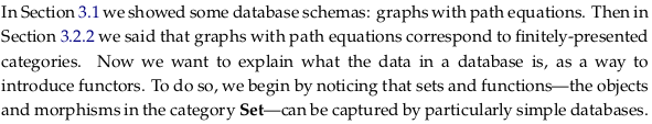
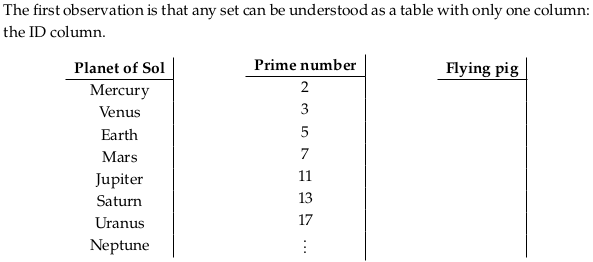
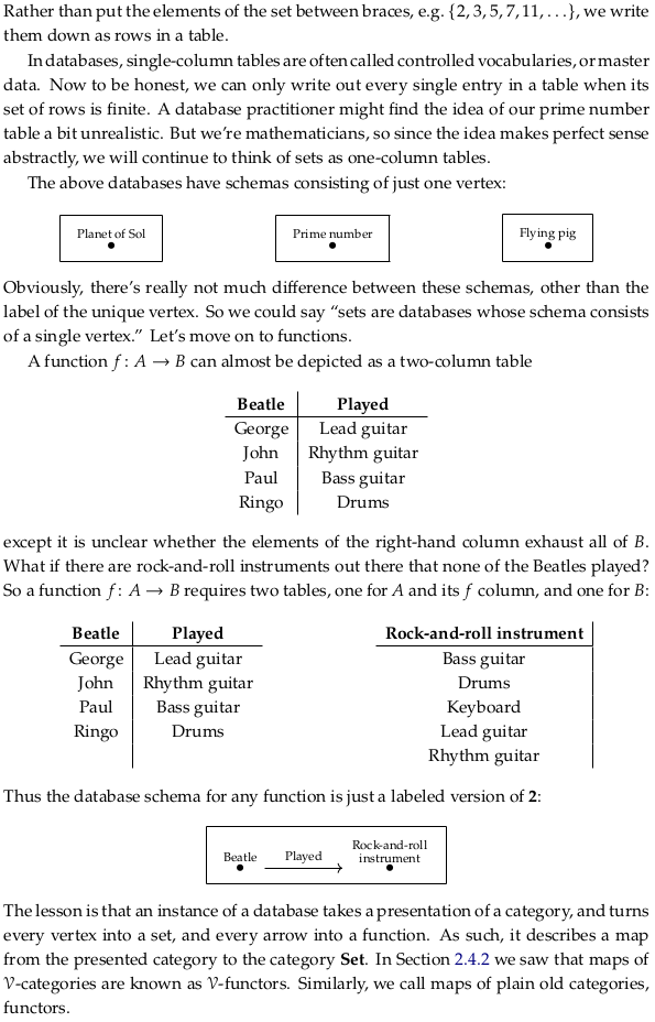
3.3.3 Database instances as Set-valued functors#
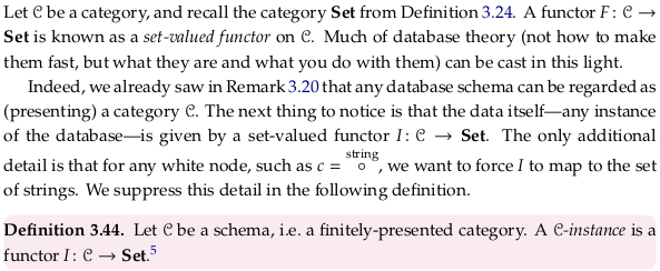

Exercise 3.45#
This function \(F_S\) will map 1 to S, and \(id_1\) to \(id_S\). It preserves identities in the one case it needs to, and it preserves composition because there is no composition to preserve.
Reveal 7S answer
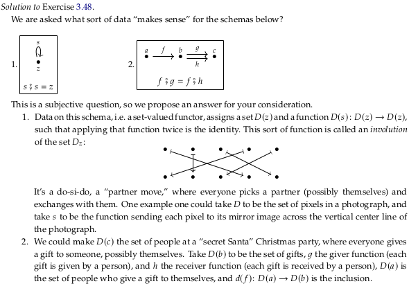
Exercise 3.48#
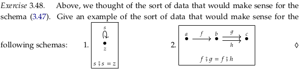
For 1., any involution. For example, if x ∈ ℝ then \(f(x) = 1/x\).
For 2., any two-stage conversion where there are two different ways to do the same thing for the
second stage. For example, working hard to make money in the first stage, then using one of two
vendors (asking the same price) to convert the money to a good.
Reveal 7S answer
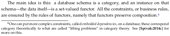
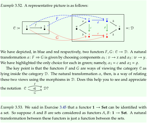
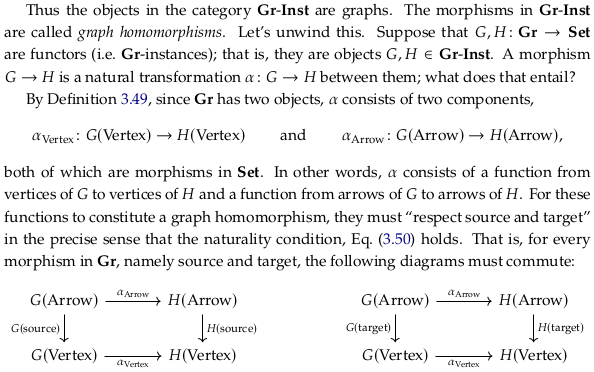
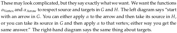
3.3.4 Natural transformations#
Prerequisite to Natural transformation (this article uses \(\eta\) for natural) and Functor category. A good way to think about a natural transformation between two functors is that we define it (its existence) in terms of its effects; because functors are like functions (defined in terms of what they do) all we can do is look at the effects (in category 𝓓). It’s similar to but opposite to defining a function in terms of data (e.g. collected data).
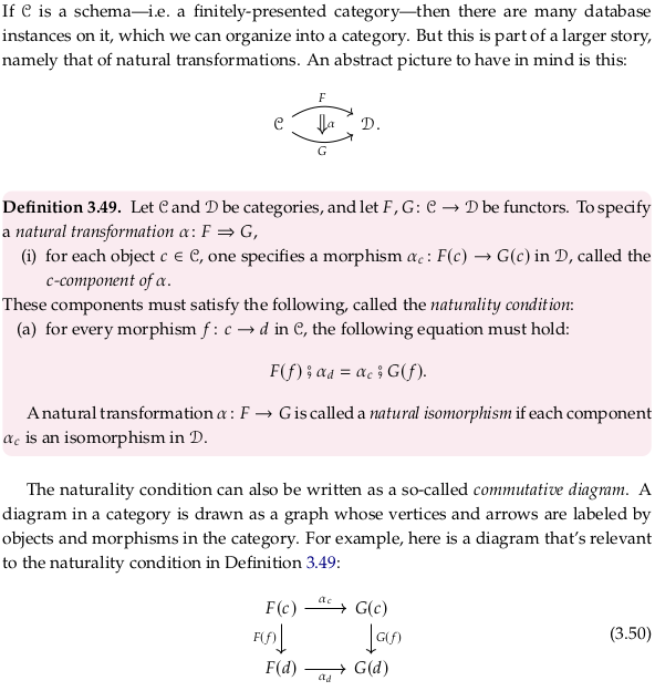
Definition 3.51.#
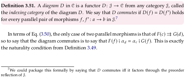
It’s not clear from this definition and the examples local to it whether Eq. (3.50) is 𝓙 or 𝓒. The following quotes from Diagram (category theory) support the former:
The diagram D is thought of as indexing a collection of objects and morphisms in C patterned on J.
Within the local context, it makes sense with the wording “the only two parallel pair of morphisms” because there are more morphisms in the example D in SSC. It also makes sense given that it must hold for every parallel pair of morphism in 𝓙; there are many more parallel paths in the 𝓓 of Example 3.52. Looking forward, this interpretation also fits the last paragraph of Definition 3.92.
Reflecting Eq. (3.50) across a diagonal to make drawing it on top of the 𝓓 of Example 3.52 easier:

Using the term “commutative” for commutative diagrams is a bit misleading; see Why are commutative diagrams called commutative diagrams? - Math SE. Said another way, the name is only related in a historical way to the term “commutative” in Commutative property.
You can use a commutative diagram to express that a particular category (say the category of real numbers) is commutative. Notice that in \(ab = ba\) that the a and b become morphisms. However, you can also use a commutative diagram to express that a particular category is associative; a commutative diagram is provided at the top of the article Associative property. Notice in the article Commutative Diagram – from Wolfram MathWorld a much shorter (and likely more memorable) version of Definition 3.28 (of an isomorphism). For a more complicated example with the diagram and algebra side-by-side, see abstract algebra - Why gives a commutative diagram a proof?.
Said another way, from soft question - Reading commutative diagrams? - Mathematics SE:
Commutative diagrams are, to put it simply, a (very) handy way of writing systems of equations in categories.
Functors are designed to transform commutative diagrams in C to commutative diagrams in D, see Functor / Properties - Wikipedia.
To draw or update commutative diagrams on Wikipedia, see Help:Displaying a formula - Commutative diagrams - Wikipedia. For documentation on tikzcd, see tikzcd: Commutative diagrams with TikZ - tikz-cd-doc.pdf.
To get started quickly, see quiver: a modern commutative diagram editor (partially selected based on star history). You can use overleaf to export the drawing, as in tikzcd export. If you have the necessary dependencies on your local machine, see tikzcd-export · GitLab.
Definition 3.54.#
In the category-theoretic view (and in some cases, the programming language view) we are looking at functions as objects (first class citizens) when we go from thinking in 𝓒 → 𝓓 to \(D^{C}\). In the database view, we are re-viewing conversions between databases (sets of tables) as objects (see the end of Exercise 3.64 below). That is, these reinterpretations happen when you step up one level of abstraction here:

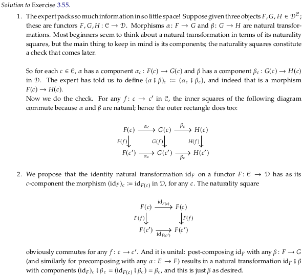
Exercise 3.55.#
For 1., say we have natural transformations α and β, and want to construct a composite ɣ. For
every c ∈ 𝓒, define \(\gamma_c = \alpha_c ⨾ \beta_c\). For a valuable proof of the naturality
condition, see the author’s answer.
For 2., the functor F maps from some category 𝓒 to 𝓓. For every c ∈ 𝓒, construct a natural
transformation via a morphism \(\iota_c: F(c) → F(c)\) in 𝓓 defined as \(id_{F(c)_{}}\). To check
unitality, we observe \(\iota_c ⨾ \alpha_c = \alpha_c\) and \(\alpha_c ⨾ \iota_c = \alpha_c\).
Reveal 7S answer

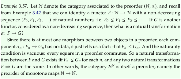
Example 3.57.#

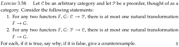
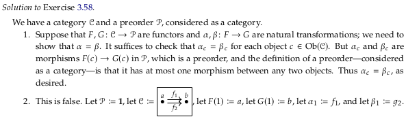
Exercise 3.58.#
For 1., this is true because a natural transformation is made up of many \(\alpha_c\) that must
exist as morphisms in 𝓟. Because we’re mapping to a preorder category, there will be at most only
choice for each of these \(\alpha_c\), meaning there will be at most one natural transformation. If
there are zero choices for any \(\alpha_c\), then the natural transformation doesn’t exist. An example
with zero choices:

For 2., this is false, taking as a counterexample the categories in Example 3.52 but adding e.g.
another option parallel to \(c\) between \(v\) and \(x\) (call it \(h\)). One could choose either \(c\) or \(h\)
to construct a natural transformation. An even smaller counterexample:

Reveal 7S answer
Remark 3.59.#
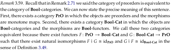
See the errata for commentary from others on this section. Read through “Definition” in Equivalence of categories for help reinterpreting it. The author is using id to refer to the identity functor in each category. The end of this section should most likely be rewritten:

An arrow category is a functor category#
Let’s try to understand the article Functor category better from one more example. From Functor category § Examples:
An arrow category \(\mathcal{C}^\rightarrow\) (whose objects are the morphisms of \({\mathcal {C}}\), and whose morphisms are commuting squares in \({\mathcal {C}}\)) is just \(\mathcal{C}^\mathbf{2}\), where 2 is the category with two objects and their identity morphisms as well as an arrow from one object to the other (but not another arrow back the other way).
See Comma category § Arrow category for that definition. Taking \(\mathcal{C}\) to be the commutative square (section 3.2.2), one functor between \(\mathbf{2}\) and \(\mathcal{C}\) is:
![]()
That is:
Which we could write as a relation as \(\{(1,A), (2,C)\}\). A short list of notable functors between these categories:
\(F = \{(1,A), (2,B)\}\)
\(G = \{(1,A), (2,C)\}\)
\(H = \{(1,B), (2,D)\}\)
\(I = \{(1,C), (2,D)\}\)
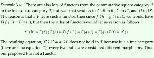
Clearly there’s a natural transformation from \(F\) to \(I\) and from \(G\) to \(H\) (and vice-versa, making both natural isomorphisms). These are the morphisms of the functor category, the natural transformations of the original category, or the commuting squares in the arrow category:
![]()
If we had taken \(\mathcal{C}\) to be the free square (section 3.2.2) then both η and ε would have been “infranatural” or “unnatural” transformations.
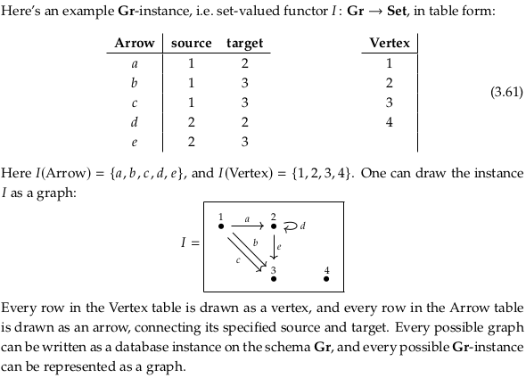
3.3.5 The category of instances on a schema#
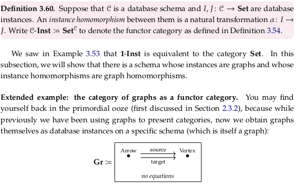
Prerequisite to Graph isomorphism.
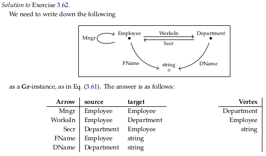
Exercise 3.62.#

Reveal 7S answer
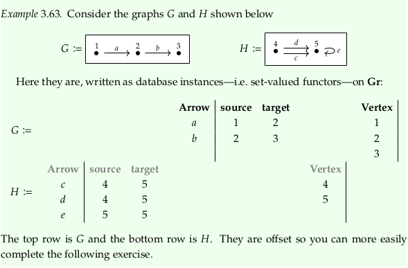
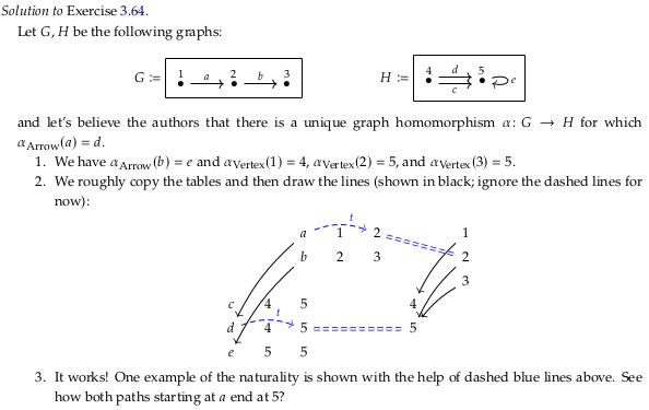
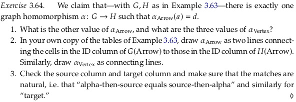
Exercise 3.64.#

Reveal 7S answer