Practice: Chp. 9

source("iplot.R")
suppressPackageStartupMessages(library(rethinking))

options(mc.cores = parallel::detectCores())

9E1. Which of the following is a requirement of the simple Metropolis algorithm?

1. The parameters must be discrete.

2. The likelihood function must be Gaussian.

3. The proposal distribution must be symmetric.

Answer. The parameters do not need to be discrete; see the top of 9.2. Metropolis algorithms and a specific example of a non-discrete parameter in section 2.4.5. Markov chain Monte Carlo.

The likelihood function does not need to be Gaussian, see the example in section 2.4.5. Markov chain Monte Carlo.

The proposal distribution needs to be symmetric. See Metropolis-Hastings algorithm and the top of 9.2. Metropolis algorithms.

9E2. Gibbs sampling is more efficient than the Metropolis algorithm. How does it achieve this extra efficiency? Are there any limitations to the Gibbs sampling strategy?

Answer. Gibbs sampling allows asymmetric proposals, which it takes advantage of by introducing adaptive proposals. An adaptive proposal is one in which the distribution of proposed parameter values adjusts intelligently. To achieve adaptive proposals it relies on conjugate priors.

One limitation to this approach is that some conjugate priors are pathological in shape. A second limitation is that these conjugate-prior based adaptive proposals don’t perform as well as HMC adaptive proposals when there are a large number of dimensions.

9E3. Which sort of parameters can Hamiltonian Monte Carlo not handle? Can you explain why?

Answer. HMC cannot handle discrete parameters. I’d guess this is because these parameters would not be differentiable. If you’re running a physics simulation, you need to be able to stop at any point.

9E4. Explain the difference between the effective number of samples, n_eff as calculated by Stan, and the actual number of samples.

Answer. All MCMC algorithms (Metropolis, Gibbs, HMC) naturally produce autocorrelated samples; see Markov chain Monte Carlo. The ‘Leapfrog steps’ and ‘Step size’ settings as described in the text help avoid this autocorrelation. The effective number of parameters reported by Stan is an estimate of the length of a Markov chain with no autocorrelation that would provide the same quality of estimate as your chain.

9E5. Which value should Rhat approach, when a chain is sampling the posterior distribution correctly?

Answer. 1.00 from above.

9E6. Sketch a good trace plot for a Markov chain, one that is effectively sampling from the posterior distribution. What is good about its shape? Then sketch a trace plot for a malfunctioning Markov chain. What about its shape indicates malfunction?

Answer. The good features of the traces in the upper plot are Stationarity, good mixing to e.g. avoid autocorrelated samples, and that all three chains stick to the same regions.

The bad features of the lower plot are just the opposite.

display_svg(file="good_trace_plot.svg", width=20, height=20)

9E7. Repeat the problem above, but now for a trace rank plot.

Answer. The good feature of the top plot is that all three chains have about the same rank histogram; they are exploring the same space.

The bad feature of the lower plot is that different chains are spending different amounts of time on the same sample values.

display_svg(file="good_trank_plot.svg", width=20, height=20)

source("practice-debug-mcmc-inference.R")

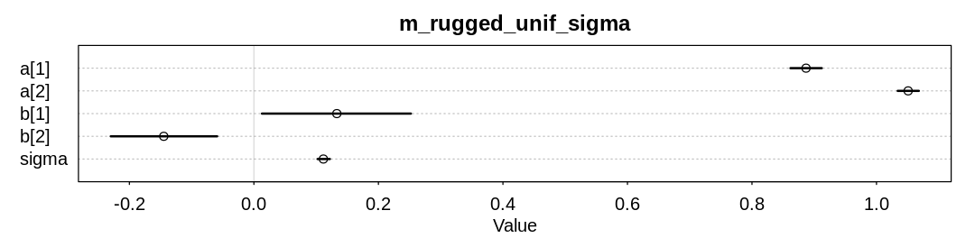
9M1. Re-estimate the terrain ruggedness model from the chapter, but now using a uniform prior for the standard deviation, sigma. The uniform prior should be dunif(0,1). Use ulam to estimate the posterior. Does the different prior have any detectible influence on the posterior distribution of sigma? Why or why not?

Answer. This change could have potentially have had an effect on the inference for sigma because it assigns zero prior probability to parameter values above 1.0. Because sigma is less than one, it doesn’t make a difference.

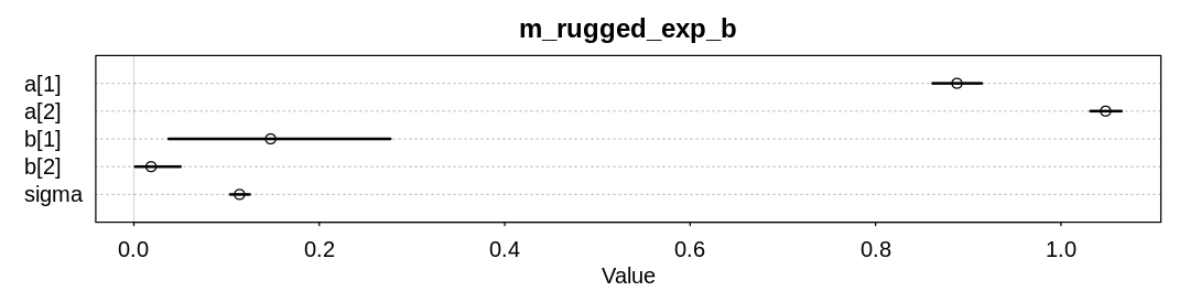
9M2. Modify the terrain ruggedness model again. This time, change the prior for b[cid] to dexp(0.3). What does this do to the posterior distribution? Can you explain it?

Answer. Notice b[2] is now positive, when previously it was inferred to be negative. Because we assigned zero prior probability to negative values, we’re forcing this new inference.

You may also see the warning message:

Warning message:
“Tail Effective Samples Size (ESS) is too low, indicating posterior variances and tail quantiles may be unreliable.
Running the chains for more iterations may help. See
http://mc-stan.org/misc/warnings.html#tail-ess”

9M3. Re-estimate one of the Stan models from the chapter, but at different numbers of warmup iterations. Be sure to use the same number of sampling iterations in each case. Compare the n_eff values. How much warmup is enough?

Answer. For the rugged models, we can get down to 200 warmup iterations and still get nearly as many effective samples as requested samples.

Warmup: 1000, Samples: 1000

Hamiltonian Monte Carlo approximation
4000 samples from 4 chains

Sampling durations (seconds):
        warmup sample total
chain:1   0.13    0.1  0.23
chain:2   0.14    0.1  0.24
chain:3   0.13    0.1  0.23
chain:4   0.13    0.1  0.23

Formula:
log_gdp_std ~ dnorm(mu, sigma)
mu <- a[cid] + b[cid] * (rugged_std - 0.215)
a[cid] ~ dnorm(1, 0.1)
b[cid] ~ dnorm(0, 0.3)
sigma ~ dexp(1)

Effective samples:

      mean       sd          5.5%        94.5%       n_eff    Rhat4    
a[1]   0.8864632 0.015808305  0.86127357  0.91186865 4861.680 0.9993934
a[2]   1.0504053 0.010061335  1.03382959  1.06629791 4825.271 0.9995729
b[1]   0.1296746 0.074197398  0.01031252  0.24994568 4850.437 1.0006880
b[2]  -0.1420051 0.056443979 -0.23200596 -0.05063607 4793.139 0.9998421
sigma  0.1117248 0.006473997  0.10178459  0.12248812 5275.691 0.9996434

recompiling to avoid crashing R session

Warmup: 500, Samples: 1000

Hamiltonian Monte Carlo approximation
4000 samples from 4 chains

Sampling durations (seconds):
        warmup sample total
chain:1   0.08   0.10  0.18
chain:2   0.08   0.10  0.18
chain:3   0.07   0.10  0.17
chain:4   0.08   0.14  0.22

Formula:
log_gdp_std ~ dnorm(mu, sigma)
mu <- a[cid] + b[cid] * (rugged_std - 0.215)
a[cid] ~ dnorm(1, 0.1)
b[cid] ~ dnorm(0, 0.3)
sigma ~ dexp(1)

Effective samples:

      mean       sd          5.5%         94.5%       n_eff    Rhat4    
a[1]   0.8871437 0.015783137  0.861933293  0.91240200 4791.376 0.9996737
a[2]   1.0503441 0.010300131  1.033947332  1.06684252 6137.590 0.9994938
b[1]   0.1330260 0.076855413  0.009644431  0.25463403 5312.412 0.9998432
b[2]  -0.1424935 0.056516607 -0.235508171 -0.05331239 5201.390 0.9993912
sigma  0.1115574 0.006139087  0.102323186  0.12156095 5391.181 0.9994400

recompiling to avoid crashing R session

Warmup: 200, Samples: 1000

Hamiltonian Monte Carlo approximation
4000 samples from 4 chains

Sampling durations (seconds):
        warmup sample total
chain:1   0.05   0.11  0.16
chain:2   0.04   0.10  0.14
chain:3   0.04   0.10  0.14
chain:4   0.04   0.10  0.14

Formula:
log_gdp_std ~ dnorm(mu, sigma)
mu <- a[cid] + b[cid] * (rugged_std - 0.215)
a[cid] ~ dnorm(1, 0.1)
b[cid] ~ dnorm(0, 0.3)
sigma ~ dexp(1)

Effective samples:

      mean       sd          5.5%        94.5%       n_eff    Rhat4    
a[1]   0.8868156 0.016386080  0.86117692  0.91257442 5515.755 0.9995938
a[2]   1.0501712 0.010276383  1.03400590  1.06691631 6522.853 0.9999509
b[1]   0.1329360 0.075514813  0.01231028  0.25272295 4785.556 0.9997946
b[2]  -0.1419804 0.054665975 -0.22770846 -0.05397096 3204.345 1.0004812
sigma  0.1114831 0.006112963  0.10230398  0.12179133 3354.359 0.9993453

9H1. Run the model below and then inspect the posterior distribution and explain what it is accomplishing.

R code 9.28

mp <- ulam(
 alist(
  a ~ dnorm(0,1),
  b ~ dcauchy(0,1)
 ), data=list(y=1) , chains=1 )

Compare the samples for the parameters a and b. Can you explain the different trace plots? If you are unfamiliar with the Cauchy distribution, you should look it up. The key feature to attend to is that it has no expected value. Can you connect this fact to the trace plot?

Warning message:
“Bulk Effective Samples Size (ESS) is too low, indicating posterior means and medians may be unreliable.
Running the chains for more iterations may help. See
https://mc-stan.org/misc/warnings.html#bulk-ess”

Warning message:
“Tail Effective Samples Size (ESS) is too low, indicating posterior variances and tail quantiles may be unreliable.
Running the chains for more iterations may help. See
https://mc-stan.org/misc/warnings.html#tail-ess”

[1] 1000
[1] 1
[1] 1000

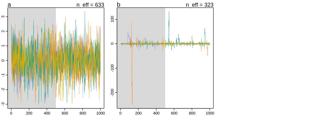
Answer. We start with two priors unconnected to the data so we’re essentially sampling from the prior rather than any posterior. Said another way, the posterior equals the prior.

The a prior is Stationary in the common sense, with a stable mean indicated by balance between the top and bottom of the figure. The Cauchy process is stationary in the sense the process statistics do not change (strictly stationary) but doesn’t have a stable mean (expected value) so doesn’t have the property sometimes referred to as wide-sense stationarity.

Without a stable mean, there is no guarantee that the Cauchy process will be symmetric vertically; large spikes towards low or high values are common in repeated simulations. The Heavy tails that define the Cauchy distribution may sometimes lead to this warning (among others):

Warning message:
“Tail Effective Samples Size (ESS) is too low, indicating posterior variances and tail quantiles may be unreliable.
Running the chains for more iterations may help. See
http://mc-stan.org/misc/warnings.html#tail-ess”

Samples from the Cauchy process sometimes to appear to display bad ‘mixing’. That is, the samples don’t appear to explore the same space as the process continues (because of the spikes). In general, the Cauchy distribution will not obey the Law of Large Numbers, that is, there’s no guarantee of convergence of the mean. Said another way, these spikes will not go away regardless of how many iterations we allow.

Because the median and mode are still defined, multiple chains may still appear to ‘converge’ to e.g. zero in this case.

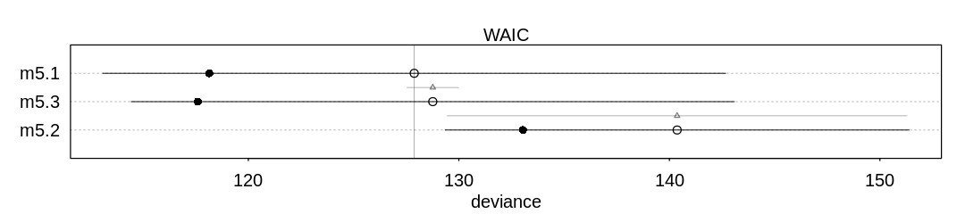
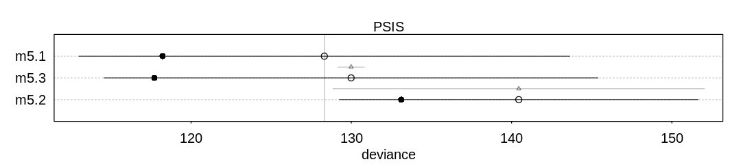
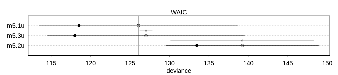
9H2. Recall the divorce rate example from Chapter 5. Repeat that analysis, using ulam this time, fitting models m5.1, m5.2, and m5.3. Use compare to compare the models on the basis of WAIC or PSIS. To use WAIC or PSIS with ulam, you need add the argument log_log=TRUE. Explain the model comparison results.

ERROR: Replace log_log in the question with log_lik

SAMPLING FOR MODEL 'bc675254cc2159bb33743bbf24468ab3' NOW (CHAIN 1).
Chain 1: 
Chain 1: Gradient evaluation took 1.4e-05 seconds
Chain 1: 1000 transitions using 10 leapfrog steps per transition would take 0.14 seconds.
Chain 1: Adjust your expectations accordingly!
Chain 1: 
Chain 1: 
Chain 1: Iteration:   1 / 1000 [  0%]  (Warmup)
Chain 1: Iteration: 100 / 1000 [ 10%]  (Warmup)
Chain 1: Iteration: 200 / 1000 [ 20%]  (Warmup)
Chain 1: Iteration: 300 / 1000 [ 30%]  (Warmup)
Chain 1: Iteration: 400 / 1000 [ 40%]  (Warmup)
Chain 1: Iteration: 500 / 1000 [ 50%]  (Warmup)
Chain 1: Iteration: 501 / 1000 [ 50%]  (Sampling)
Chain 1: Iteration: 600 / 1000 [ 60%]  (Sampling)
Chain 1: Iteration: 700 / 1000 [ 70%]  (Sampling)
Chain 1: Iteration: 800 / 1000 [ 80%]  (Sampling)
Chain 1: Iteration: 900 / 1000 [ 90%]  (Sampling)
Chain 1: Iteration: 1000 / 1000 [100%]  (Sampling)
Chain 1: 
Chain 1:  Elapsed Time: 0.018729 seconds (Warm-up)
Chain 1:                0.017549 seconds (Sampling)
Chain 1:                0.036278 seconds (Total)
Chain 1: 

SAMPLING FOR MODEL '8b690dbf8986a1e80daeae2b8293f78f' NOW (CHAIN 1).
Chain 1: 
Chain 1: Gradient evaluation took 1.1e-05 seconds
Chain 1: 1000 transitions using 10 leapfrog steps per transition would take 0.11 seconds.
Chain 1: Adjust your expectations accordingly!
Chain 1: 
Chain 1: 
Chain 1: Iteration:   1 / 1000 [  0%]  (Warmup)
Chain 1: Iteration: 100 / 1000 [ 10%]  (Warmup)
Chain 1: Iteration: 200 / 1000 [ 20%]  (Warmup)
Chain 1: Iteration: 300 / 1000 [ 30%]  (Warmup)
Chain 1: Iteration: 400 / 1000 [ 40%]  (Warmup)
Chain 1: Iteration: 500 / 1000 [ 50%]  (Warmup)
Chain 1: Iteration: 501 / 1000 [ 50%]  (Sampling)
Chain 1: Iteration: 600 / 1000 [ 60%]  (Sampling)
Chain 1: Iteration: 700 / 1000 [ 70%]  (Sampling)
Chain 1: Iteration: 800 / 1000 [ 80%]  (Sampling)
Chain 1: Iteration: 900 / 1000 [ 90%]  (Sampling)
Chain 1: Iteration: 1000 / 1000 [100%]  (Sampling)
Chain 1: 
Chain 1:  Elapsed Time: 0.019359 seconds (Warm-up)
Chain 1:                0.018097 seconds (Sampling)
Chain 1:                0.037456 seconds (Total)
Chain 1: 

SAMPLING FOR MODEL 'd27a7128c546624a07b356f67a87a125' NOW (CHAIN 1).
Chain 1: 
Chain 1: Gradient evaluation took 2e-05 seconds
Chain 1: 1000 transitions using 10 leapfrog steps per transition would take 0.2 seconds.
Chain 1: Adjust your expectations accordingly!
Chain 1: 
Chain 1: 
Chain 1: Iteration:   1 / 1000 [  0%]  (Warmup)
Chain 1: Iteration: 100 / 1000 [ 10%]  (Warmup)
Chain 1: Iteration: 200 / 1000 [ 20%]  (Warmup)
Chain 1: Iteration: 300 / 1000 [ 30%]  (Warmup)
Chain 1: Iteration: 400 / 1000 [ 40%]  (Warmup)
Chain 1: Iteration: 500 / 1000 [ 50%]  (Warmup)
Chain 1: Iteration: 501 / 1000 [ 50%]  (Sampling)
Chain 1: Iteration: 600 / 1000 [ 60%]  (Sampling)
Chain 1: Iteration: 700 / 1000 [ 70%]  (Sampling)
Chain 1: Iteration: 800 / 1000 [ 80%]  (Sampling)
Chain 1: Iteration: 900 / 1000 [ 90%]  (Sampling)
Chain 1: Iteration: 1000 / 1000 [100%]  (Sampling)
Chain 1: 
Chain 1:  Elapsed Time: 0.040591 seconds (Warm-up)
Chain 1:                0.03395 seconds (Sampling)
Chain 1:                0.074541 seconds (Total)
Chain 1: 

Some Pareto k values are very high (>1). Set pointwise=TRUE to inspect individual points.

Some Pareto k values are high (>0.5). Set pointwise=TRUE to inspect individual points.

Some Pareto k values are very high (>1). Set pointwise=TRUE to inspect individual points.

Models fit using ulam:

Some Pareto k values are high (>0.5). Set pointwise=TRUE to inspect individual points.

Some Pareto k values are high (>0.5). Set pointwise=TRUE to inspect individual points.

Answer. In Chapter 5, further analysis showed the DAG describing these three variables was most likely D <- A -> M. This fits the poor performance of the model (m5.2) which is making predictions based on only M; it only has indirect information (through A) to predict D.

The unnecessary additional predictor M is likely hurting the predictive performance of the multiple regression model (m5.3). Without a lot of data it’s likely we’re only overfitting to the noise in M rather than gaining any predictive accuracy from it (see AIC’s parameter penalty).

9H3. Sometimes changing a prior for one parameter has unanticipated effects on other parameters. This is because when a parameter is highly correlated with another parameter in the posterior, the prior influences both parameters. Here’s an example to work and think through.

Go back to the leg length example in Chapter 6 and use the code there to simulate height and leg lengths for 100 imagined individuals. Below is the model you fit before, resulting in a highly correlated posterior for the two beta parameters. This time, fit the model using ulam:

R code 9.29

m5.8s <- ulam(
 alist(
  height ~ dnorm( mu , sigma ) ,
  mu <- a + bl*leg_left + br*leg_right ,
  a ~ dnorm( 10 , 100 ) ,
  bl ~ dnorm( 2 , 10 ) ,
  br ~ dnorm( 2 , 10 ) ,
  sigma ~ dexp( 1 )
 ) , data=d, chains=4,
 start=list(a=10,bl=0,br=0.1,sigma=1) )

Compare the posterior distribution produced by the code above to the posterior distribution produced when you change the prior for br so that it is strictly positive:

R code 9.30

m5.8s2 <- ulam(
 alist(
  height ~ dnorm( mu , sigma ) ,
  mu <- a + bl*leg_left + br*leg_right ,
  a ~ dnorm( 10 , 100 ) ,
  bl ~ dnorm( 2 , 10 ) ,
  br ~ dnorm( 2 , 10 ) ,
  sigma ~ dexp( 1 )
 ) , data=d, chains=4,
 constraints=list(br='lower=0'),
 start=list(a=10,bl=0,br=0.1,sigma=1) )

Note the constraints list. What this does is constrain the prior distribution of br so that it has positive probability only above zero. In other words, that prior ensures that the posterior distribution for br will have no probability mass below zero. Compare the two posterior distributions for m5.8s and m5.8s2. What has changed in the posterior distribution of both beta parameters? Can you explain the change induced by the change in prior?

ERROR: These model names should be based on m6.1 rather than m5.8.

source('simulate-height-leg-lengths.R')

## R code 9.29
m5.8s <- ulam(
  alist(
    height ~ dnorm(mu, sigma),
    mu <- a + bl * leg_left + br * leg_right,
    a ~ dnorm(10, 100),
    bl ~ dnorm(2, 10),
    br ~ dnorm(2, 10),
    sigma ~ dexp(1)
  ),
  data = d, chains = 4, cores = 4,
  log_lik = TRUE,
  start = list(a = 10, bl = 0, br = 0.1, sigma = 1)
)

## R code 9.30
m5.8s2 <- ulam(
  alist(
    height ~ dnorm(mu, sigma),
    mu <- a + bl * leg_left + br * leg_right,
    a ~ dnorm(10, 100),
    bl ~ dnorm(2, 10),
    br ~ dnorm(2, 10),
    sigma ~ dexp(1)
  ),
  data = d, chains = 4, cores = 4,
  log_lik = TRUE,
  constraints = list(br = "lower=0"),
  start = list(a = 10, bl = 0, br = 0.1, sigma = 1)
)

iplot(function() {
  plot(precis(m5.8s), main="m5.8s")
}, ar=4.0)

iplot(function() {
  plot(precis(m5.8s2), main="m5.8s2")
}, ar=4.0)

Warning message:
“There were 1142 transitions after warmup that exceeded the maximum treedepth. Increase max_treedepth above 10. See
https://mc-stan.org/misc/warnings.html#maximum-treedepth-exceeded”

Warning message:
“Examine the pairs() plot to diagnose sampling problems
”

Warning message:
“There were 6 divergent transitions after warmup. See
https://mc-stan.org/misc/warnings.html#divergent-transitions-after-warmup
to find out why this is a problem and how to eliminate them.”

Warning message:
“There were 1200 transitions after warmup that exceeded the maximum treedepth. Increase max_treedepth above 10. See
https://mc-stan.org/misc/warnings.html#maximum-treedepth-exceeded”

Warning message:
“Examine the pairs() plot to diagnose sampling problems
”

Warning message:
“Bulk Effective Samples Size (ESS) is too low, indicating posterior means and medians may be unreliable.
Running the chains for more iterations may help. See
https://mc-stan.org/misc/warnings.html#bulk-ess”

Warning message:
“Tail Effective Samples Size (ESS) is too low, indicating posterior variances and tail quantiles may be unreliable.
Running the chains for more iterations may help. See
https://mc-stan.org/misc/warnings.html#tail-ess”

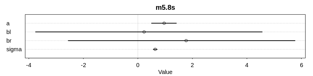
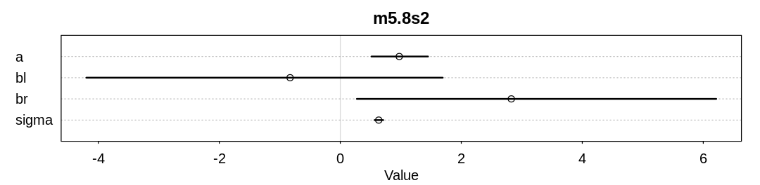
Answer. The \(\beta_l\) parameter inference has adjusted to the \(\beta_r\) prior by becoming negative.

9H4. For the two models fit in the previous problem, use WAIC or PSIS to compare the effective numbers of parameters for each model. You will need to use log_lik=TRUE to instruct ulam to compute the terms that both WAIC and PSIS need. Which model has more effective parameters? Why?

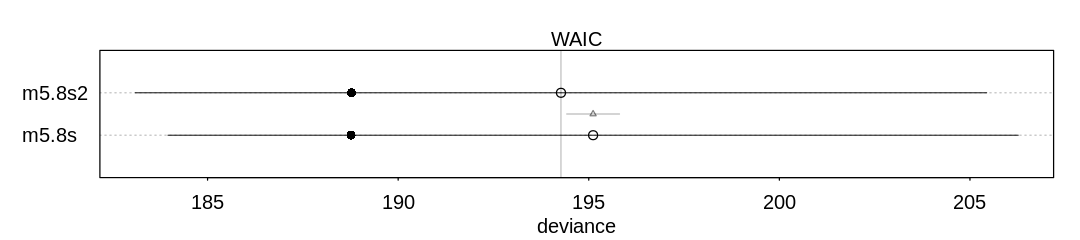
Answer. The first model (m5.8s) has more effective parameters. The number of effective parameters is based on variance in the posterior. By adding a prior we’ve apparently limited the overfitting to noise that happens in the first model, leading to less variance in both \(\beta_l\) and \(\beta_r\) and therefore less variance in the posterior.

iplot(function() {
  plot(compare(m5.8s, m5.8s2))
}, ar=4.5)

display_markdown("m5.8s:")
display(WAIC(m5.8s), mimetypes="text/plain")

display_markdown("<br/> m5.8s2:")
display(WAIC(m5.8s2), mimetypes="text/plain")

# post <- extract.samples(m5.8s2)
# n_samples <- 1000
# logprob <- sapply(1:n_samples,
#   function(s) {
#     mu <- post$a[s] + post$bl[s]*d$leg_left + post$br[s]*d$leg_right
#     dnorm(d$height, mu, post$sigma[s], log=TRUE)
#   }
# )
# n_cases <- nrow(d)
# pWAIC <- sapply(1:n_cases, function(i) var(logprob[i,]) )
# display(sum(pWAIC))

m5.8s:

  WAIC    lppd      penalty  std_err
1 195.114 -94.38185 3.175155 11.1535

m5.8s2:

  WAIC     lppd      penalty  std_err 
1 194.2712 -94.38758 2.748007 11.16886

source('practice-metropolis-islands.R')
source('practice-metropolis-globe-tossing.R')

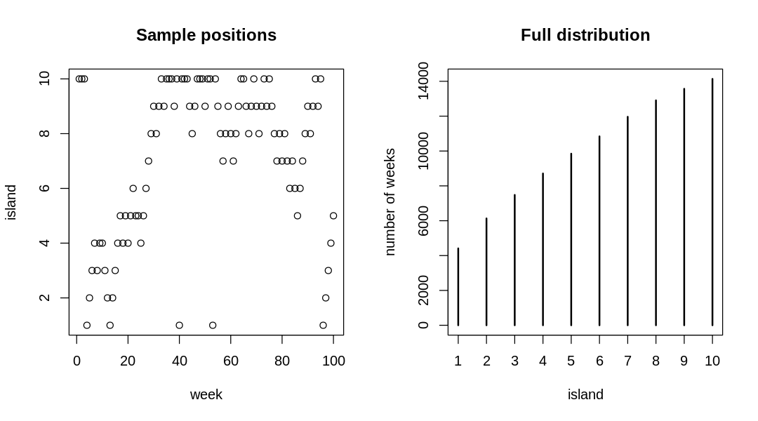
9H5. Modify the Metropolis algorithm code from the chapter to handle the case that the island populations have a different distribution than the island labels. This means the island’s number will not be the same as its population.

Answer. The new island populations are proportional to:

island_pop_prop = sqrt(island_number)

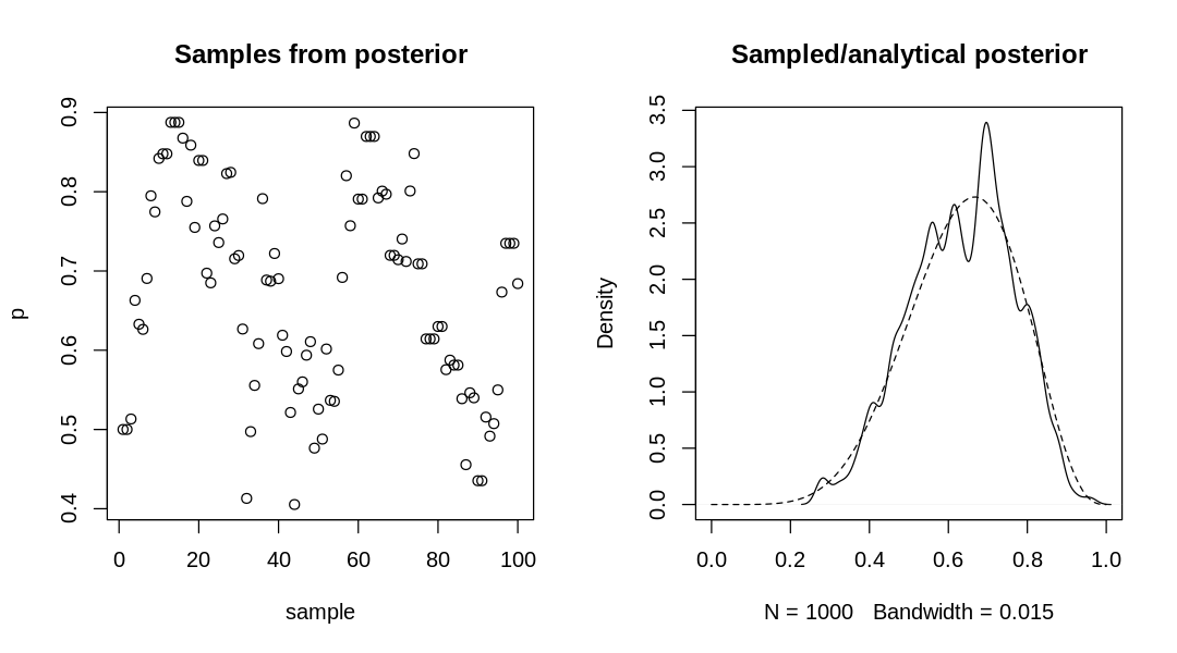
9H6. Modify the Metropolis algorithm code from the chapter to write your own simple MCMC estimator for globe tossing data and model from Chapter 2.

Answer. See R code 2.8, which provides most of the answer.

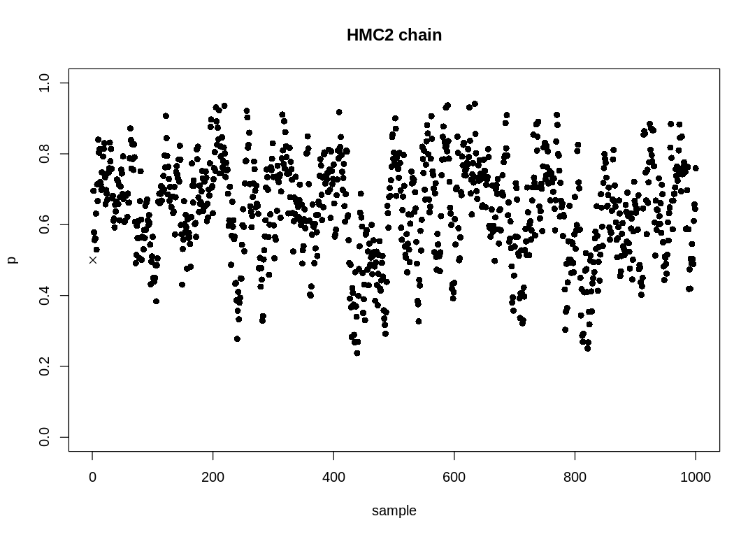
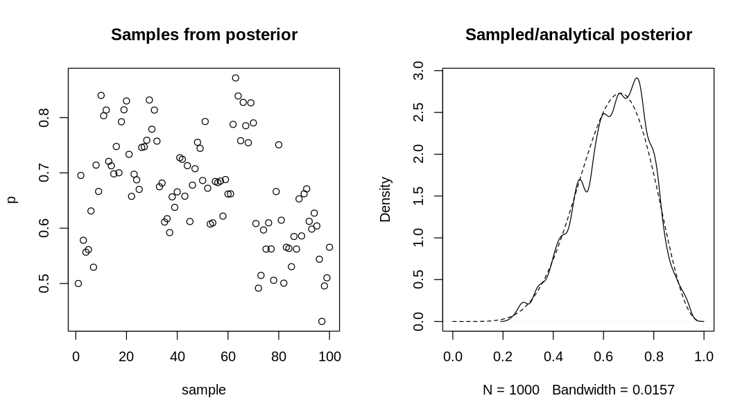
9H7. Can you write your own Hamiltonian Monte Carlo algorithm for the globe tossing data, using the R code in the chapter? You will have to write your own functions for the likelihood and gradient, but you can use the HMC2 function.

Answer. The probability mass function for the binomial distribution is defined as:

\[ f(p, k, n) = \binom{n}{k}p^k(1-p)^{n-k} \]

Taking the logarithm:

\[\begin{split} \begin{align} g(p, k, n) & = log(f(p, k, n)) = log\left(\binom{n}{k}p^k(1-p)^{n-k}\right) \\ g(p, k, n) & = log\left(\binom{n}{k}\right) + k·log(p) + (n-k)·log(1-p) \end{align} \end{split}\]

And the derivative with respect to \(p\):

\[\begin{split} \begin{align} \frac{\partial g(p, k, n)}{\partial p} & = \frac{\partial log\left(\binom{n}{k}\right)}{\partial p} + \frac{\partial k·log(p)}{\partial p} + \frac{\partial z(p,k,n)}{\partial p} \\ z(p, k, n) & = (n -k)·log(y) \\ y(p) & = 1 - p \\ \end{align} \end{split}\]

Notice that:

\[\begin{split} \begin{align} \frac{\partial z(p, k, n)}{\partial y} & = \frac{n -k}{y} \\ \frac{\partial y(p)}{\partial p} & = -1 \end{align} \end{split}\]

So that:

\[\begin{split} \begin{align} \frac{\partial g(p, k, n)}{\partial p} & = 0 + k/p + \frac{\partial z}{\partial y}\frac{\partial y}{\partial p} \\ \frac{\partial g(p, k, n)}{\partial p} & = k/p + \frac{n - k}{p - 1} \end{align} \end{split}\]

To partially verify the above in sympy:

p, n, k = symbols('p n k')
diff(log(p**k) - log((1-p)**(n-k)), p)

source('practice-hmc-globe-tossing.R')