Practice: Chp. 14#
source("iplot.R")
suppressPackageStartupMessages(library(rethinking))
14E1. Add to the following model varying slopes on the predictor x.
Answer. See section 14.1.3. Notice the distinction of \(i\) and \(j\) indexes.
14E2. Think up a context in which varying intercepts will be positively correlated with varying slopes. Provide a mechanistic explanation for the correlation.
Answer. If you believe that education leads to greater wealth, then in the prediction of wealth based on parent’s wealth. If you come from family with a lot of money you’ll start off with a lot of money (the intercept), and because wealth builds on wealth the addition of education will help more than for someone who doesn’t have as many resources to work with to start (the slope). You could replace education with ambition or something else along that theme, as well.
We could also adapt the cafe example to use an M indicator (for morning) rather than an A
indicator for afternoon. The intercepts would have to become the afternoon wait. Long afternoon
waits are correlated with even longer morning waits.
14E3. When is it possible for a varying slopes model to have fewer effective parameters (as estimated by WAIC or PSIS) than the corresponding model with fixed (unpooled) slopes? Explain.
Answer. When there is some relationship between the intercepts and slopes that helps the model regularize itself. That is, if there is some correlation between intercepts and slopes, the model should be able to detect this and effectively learn to predict intercepts from slopes, and vice versa. This is similar to how in an intercepts-only multilevel model knowing some intercepts should help the model predict other intercepts; the known intercepts are a regularizing prior for new intercepts.
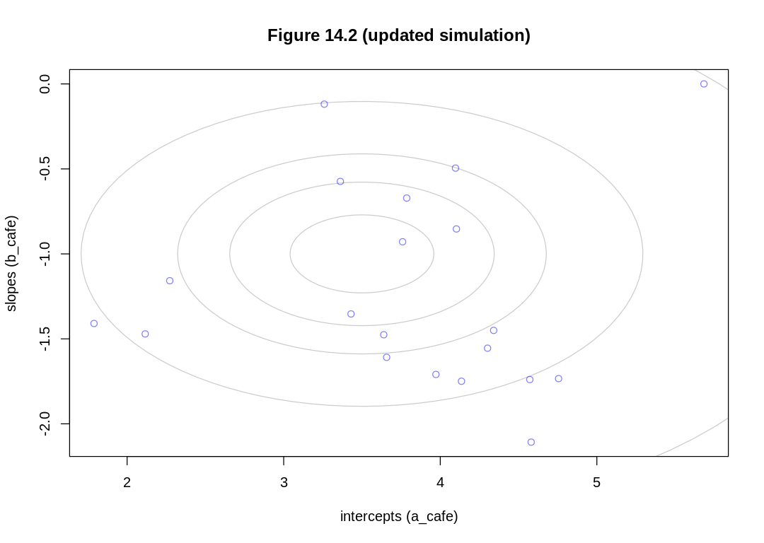
14M1. Repeat the café robot simulation from the beginning of the chapter. This time, set rho
to zero, so that there is no correlation between intercepts and slopes. How does the posterior
distribution of the correlation reflect this change in the underlying simulation?
Answer. Rerun the simulation:
a <- 3.5 # average morning wait time
b <- (-1) # average difference afternoon wait time
sigma_a <- 1 # std dev in intercepts
sigma_b <- 0.5 # std dev in slopes
rho <- (-0.0) # correlation between intercepts and slopes

Mu <- c(a, b)

sigmas <- c(sigma_a, sigma_b) # standard deviations
Rho <- matrix(c(1, rho, rho, 1), nrow = 2) # correlation matrix
Sigma <- diag(sigmas) %*% Rho %*% diag(sigmas)

N_cafes <- 20

library(MASS)
set.seed(5) # used to replicate example
vary_effects <- mvrnorm(N_cafes, Mu, Sigma)

a_cafe <- vary_effects[, 1]
b_cafe <- vary_effects[, 2]

iplot(function() {
  plot(a_cafe, b_cafe,
    col = rangi2,
    xlab = "intercepts (a_cafe)", ylab = "slopes (b_cafe)",
    main = "Figure 14.2 (updated simulation)"
  )

  library(ellipse)
  for (l in c(0.1, 0.3, 0.5, 0.8, 0.99)) {
    lines(ellipse(Sigma, centre = Mu, level = l), col = col.alpha("black", 0.2))
  }
})

set.seed(22)
N_visits <- 10
afternoon <- rep(0:1, N_visits * N_cafes / 2)
cafe_id <- rep(1:N_cafes, each = N_visits)
mu <- a_cafe[cafe_id] + b_cafe[cafe_id] * afternoon
sigma <- 0.5 # std dev within cafes
wait <- rnorm(N_visits * N_cafes, mu, sigma)
d <- data.frame(cafe = cafe_id, afternoon = afternoon, wait = wait)
Attaching package: ‘ellipse’
The following object is masked from ‘package:rethinking’:

    pairs
The following object is masked from ‘package:graphics’:

    pairs
Refit the model:
set.seed(867530)
m_cafe_rho_zero <- ulam(
  alist(
    wait ~ normal(mu, sigma),
    mu <- a_cafe[cafe] + b_cafe[cafe] * afternoon,
    c(a_cafe, b_cafe)[cafe] ~ multi_normal(c(a, b), Rho, sigma_cafe),
    a ~ normal(5, 2),
    b ~ normal(-1, 0.5),
    sigma_cafe ~ exponential(1),
    sigma ~ exponential(1),
    Rho ~ lkj_corr(2)
  ),
  data = d, chains = 4, cores = 4
)
display(precis(m_cafe_rho_zero, depth = 3), mimetypes="text/plain")

post <- extract.samples(m_cafe_rho_zero) # posterior
R <- rlkjcorr(1e4, K = 2, eta = 2) # prior

iplot(function() {
  dens(post$Rho[, 1, 2], xlim = c(-1, 1))
  dens(R[, 1, 2], add = TRUE, lty = 2)
})
              mean        sd           5.5%       94.5%      n_eff    Rhat4
b_cafe[1]     -0.97493827 2.706508e-01 -1.4053396 -0.5321296 2558.033 0.9985400
b_cafe[2]     -1.57678103 2.754448e-01 -2.0302763 -1.1429525 2258.533 0.9987245
b_cafe[3]     -1.75208873 2.937009e-01 -2.2155046 -1.2700634 2475.211 1.0004769
b_cafe[4]     -1.38179526 2.640233e-01 -1.7984554 -0.9628625 2678.364 0.9997784
b_cafe[5]     -0.85552684 2.673436e-01 -1.2846377 -0.4451974 2146.033 0.9990816
b_cafe[6]     -1.03052158 2.727011e-01 -1.4647225 -0.5959246 2341.112 1.0009258
b_cafe[7]     -1.07318113 2.612501e-01 -1.5018916 -0.6632712 2523.437 0.9998771
b_cafe[8]     -1.66622936 2.724191e-01 -2.1166805 -1.2528713 2411.146 1.0007548
b_cafe[9]     -1.09643654 2.628003e-01 -1.5073631 -0.6833408 2509.108 0.9986496
b_cafe[10]    -0.85150181 2.644251e-01 -1.2527569 -0.4179187 2583.283 0.9994003
b_cafe[11]    -0.94436493 2.765405e-01 -1.3854714 -0.4974285 2568.146 0.9985809
b_cafe[12]    -1.08532110 2.689619e-01 -1.5141136 -0.6673375 2766.285 1.0006618
b_cafe[13]    -1.82885505 2.764952e-01 -2.2718830 -1.3952793 2499.467 0.9990739
b_cafe[14]    -1.09088505 2.773739e-01 -1.5262770 -0.6556258 2419.601 0.9986678
b_cafe[15]    -2.08013935 2.922605e-01 -2.5285539 -1.6230970 2367.273 1.0003216
b_cafe[16]    -1.13964911 2.668720e-01 -1.5497444 -0.7027246 2683.230 0.9985100
b_cafe[17]    -0.84962462 2.791103e-01 -1.2910448 -0.4098209 2627.050 1.0004932
b_cafe[18]     0.13329806 2.973738e-01 -0.3546918  0.6137691 2271.025 0.9996235
b_cafe[19]    -0.05123218 2.914838e-01 -0.5206416  0.4161668 2227.332 0.9997787
b_cafe[20]    -0.94603730 2.643219e-01 -1.3730128 -0.5212390 2253.346 0.9992708
a_cafe[1]      4.32822010 2.020550e-01  3.9961308  4.6447876 2655.898 0.9990083
a_cafe[2]      2.23007232 2.012716e-01  1.9124224  2.5524646 2430.606 0.9988290
a_cafe[3]      4.55863435 2.128146e-01  4.2177601  4.8939822 2441.837 1.0012199
a_cafe[4]      3.31432538 1.956863e-01  2.9999354  3.6215312 2700.695 0.9993147
a_cafe[5]      1.92490907 1.986681e-01  1.6207611  2.2437742 2374.147 0.9986663
a_cafe[6]      4.24067936 1.990592e-01  3.9296951  4.5483649 2351.843 0.9995529
a_cafe[7]      3.77722779 1.908971e-01  3.4746905  4.0842010 2392.385 0.9998529
a_cafe[8]      4.12167102 2.033142e-01  3.8058353  4.4586906 2764.740 1.0017864
a_cafe[9]      3.91765196 1.923953e-01  3.6088796  4.2293424 2563.342 0.9989676
a_cafe[10]     3.46479236 2.000028e-01  3.1430532  3.7814975 2343.924 0.9993257
a_cafe[11]     1.95604246 2.003907e-01  1.6292569  2.2770210 2497.175 0.9988287
a_cafe[12]     3.98535177 1.923491e-01  3.6838910  4.2991258 2487.950 0.9997389
a_cafe[13]     4.14900451 2.017190e-01  3.8299155  4.4610220 2534.936 0.9989087
a_cafe[14]     3.31122820 2.030783e-01  2.9852590  3.6312353 2594.142 0.9994834
a_cafe[15]     4.62640653 2.048657e-01  4.3016374  4.9457133 2585.030 1.0030749
a_cafe[16]     3.48916086 1.981373e-01  3.1825172  3.8082679 2782.811 1.0004568
a_cafe[17]     4.13659311 2.049720e-01  3.8173995  4.4642264 2521.503 0.9996007
a_cafe[18]     5.57907198 2.139529e-01  5.2380410  5.9266490 2419.397 0.9987837
a_cafe[19]     3.07139300 2.068774e-01  2.7288774  3.4107189 2409.187 0.9994801
a_cafe[20]     3.72791143 1.933597e-01  3.4257859  4.0296822 2214.056 0.9992702
a              3.70381547 2.298564e-01  3.3455440  4.0634464 2344.457 1.0003163
b             -1.09575262 1.568141e-01 -1.3393037 -0.8450130 2020.744 0.9996859
sigma_cafe[1]  0.98523622 1.841260e-01  0.7384284  1.3121756 2191.504 1.0001043
sigma_cafe[2]  0.63873123 1.387958e-01  0.4412895  0.8792464 1888.167 0.9996571
sigma          0.47388432 2.663314e-02  0.4333083  0.5167588 2110.001 0.9995346
Rho[1,1]       1.00000000 0.000000e+00  1.0000000  1.0000000      NaN       NaN
Rho[1,2]      -0.04711170 2.294524e-01 -0.4003752  0.3325041 1973.052 0.9995424
Rho[2,1]      -0.04711170 2.294524e-01 -0.4003752  0.3325041 1973.052 0.9995424
Rho[2,2]       1.00000000 9.264531e-17  1.0000000  1.0000000 1999.376 0.9979980
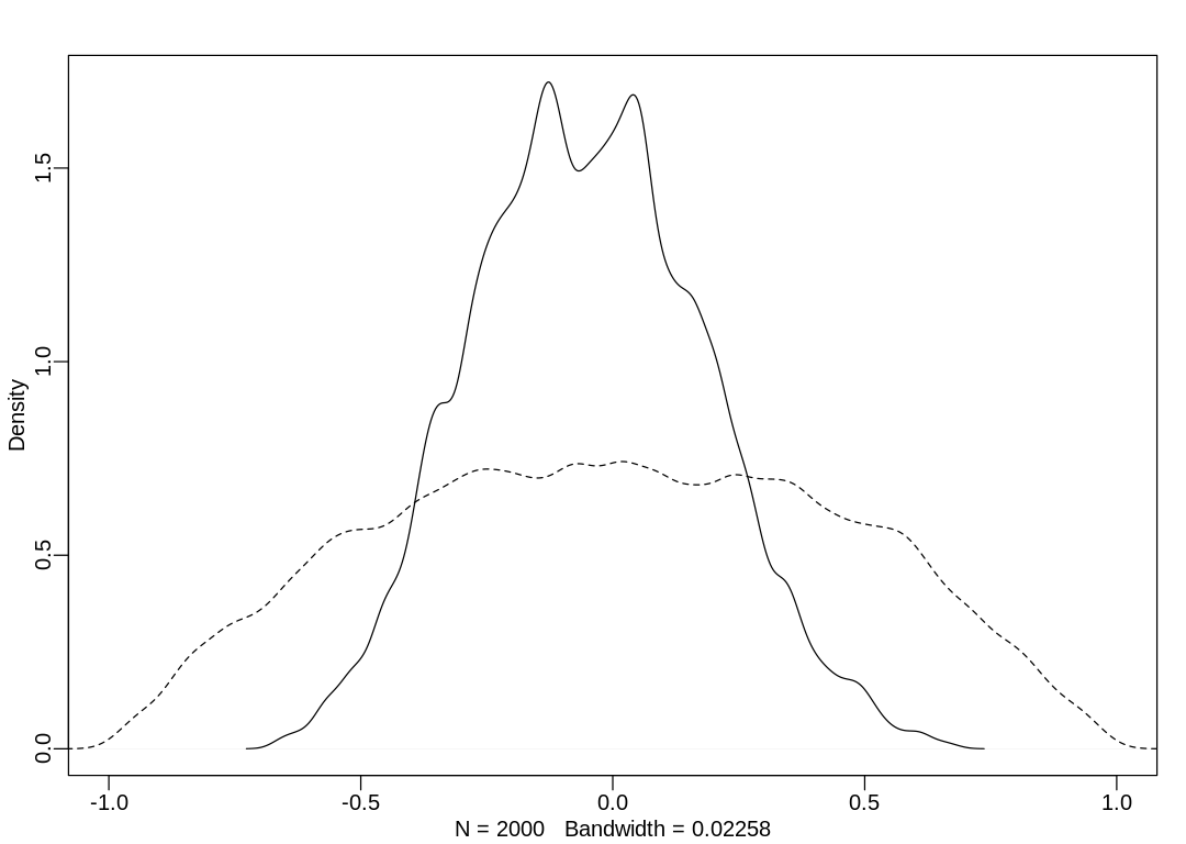
The model has inferred rho is zero, as expected.
14M2. Fit this multilevel model to the simulated café data:
Use WAIC to compare this model to the model from the chapter, the one that uses a multi-variate Gaussian prior. Explain the result.
a <- 3.5 # average morning wait time
b <- (-1) # average difference afternoon wait time
sigma_a <- 1 # std dev in intercepts
sigma_b <- 0.5 # std dev in slopes
rho <- (-0.7) # correlation between intercepts and slopes

Mu <- c(a, b)

sigmas <- c(sigma_a, sigma_b) # standard deviations
Rho <- matrix(c(1, rho, rho, 1), nrow = 2) # correlation matrix
Sigma <- diag(sigmas) %*% Rho %*% diag(sigmas)

N_cafes <- 20

library(MASS)
set.seed(5) # used to replicate example
vary_effects <- mvrnorm(N_cafes, Mu, Sigma)

a_cafe <- vary_effects[, 1]
b_cafe <- vary_effects[, 2]

set.seed(22)
N_visits <- 10
afternoon <- rep(0:1, N_visits * N_cafes / 2)
cafe_id <- rep(1:N_cafes, each = N_visits)
mu <- a_cafe[cafe_id] + b_cafe[cafe_id] * afternoon
sigma <- 0.5 # std dev within cafes
wait <- rnorm(N_visits * N_cafes, mu, sigma)
d <- data.frame(cafe = cafe_id, afternoon = afternoon, wait = wait)

m_cafe_separate_variation <- ulam(
  alist(
    wait ~ normal(mu, sigma),
    mu <- a_cafe[cafe] + b_cafe[cafe] * afternoon,
    a_cafe[cafe] ~ normal(a, sigma_a),
    b_cafe[cafe] ~ normal(b, sigma_b),
    a ~ normal(5, 2),
    b ~ normal(-1, 0.5),
    sigma ~ exponential(1),
    sigma_a ~ exponential(1),
    sigma_b ~ exponential(1)
  ),
  data = d, chains = 4, cores = 4, log_lik = TRUE
)

m14.1 <- ulam(
  alist(
    wait ~ normal(mu, sigma),
    mu <- a_cafe[cafe] + b_cafe[cafe] * afternoon,
    c(a_cafe, b_cafe)[cafe] ~ multi_normal(c(a, b), Rho, sigma_cafe),
    a ~ normal(5, 2),
    b ~ normal(-1, 0.5),
    sigma_cafe ~ exponential(1),
    sigma ~ exponential(1),
    Rho ~ lkj_corr(2)
  ),
  data = d, chains = 4, cores = 4, log_lik = TRUE
)
Answer. A compare plot with its associated raw data:
iplot(function() {
  plot(compare(m14.1, m_cafe_separate_variation))
}, ar=4.5)
display_markdown("Raw data (preceding plot):")
display(compare(m14.1, m_cafe_separate_variation), mimetypes="text/plain")
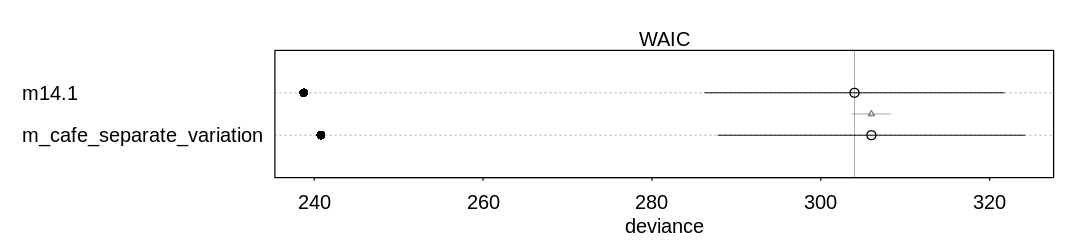
Raw data (preceding plot):
                          WAIC     SE       dWAIC    dSE     pWAIC    weight
m14.1                     303.9898 17.71746 0.000000      NA 32.61315 0.731242
m_cafe_separate_variation 305.9916 18.16013 2.001866 2.29854 32.59902 0.268758
The new model fits the training data worse (as expected, having fewer parameters). It doesn’t make up for this in the penalty term, though, because it also does less parameter sharing.
14M3. Re-estimate the varying slopes model for the UCBadmit data, now using a non-centered
parameterization. Compare the efficiency of the forms of the model, using n_eff. Which is better?
Which chain sampled faster?
ERROR. There is no varying slopes model for UCBadmit data. This is the first chapter on
varying slopes, and no model in this chapter is based on that dataset.
It’s likely the non-centered parameterization does better, if we had what model the author is referring to.
14M4. Use WAIC to compare the Gaussian process model of Oceanic tools to the models fit to the same data in Chapter 11. Pay special attention to the effective numbers of parameters, as estimated by WAIC.
Answer. Let’s reproduce results from the two chapters:
data(islandsDistMatrix)
data(Kline2) # load the ordinary data, now with coordinates
d <- Kline2
d$P <- scale(log(d$population))
d$contact_id <- ifelse(d$contact == "high", 2, 1)

dat <- list(
  T = d$total_tools,
  P = d$P,
  cid = d$contact_id
)

# intercept only
m11.9 <- ulam(
  alist(
    T ~ dpois(lambda),
    log(lambda) <- a,
    a ~ dnorm(3, 0.5)
  ),
  data = dat, chains = 4, log_lik = TRUE
)

# interaction model
m11.10 <- ulam(
  alist(
    T ~ dpois(lambda),
    log(lambda) <- a[cid] + b[cid] * P,
    a[cid] ~ dnorm(3, 0.5),
    b[cid] ~ dnorm(0, 0.2)
  ),
  data = dat, chains = 4, log_lik = TRUE
)

dat2 <- list(T = d$total_tools, P = d$population, cid = d$contact_id)
m11.11 <- ulam(
  alist(
    T ~ dpois(lambda),
    lambda <- exp(a[cid]) * P^b[cid] / g,
    a[cid] ~ dnorm(1, 1),
    b[cid] ~ dexp(1),
    g ~ dexp(1)
  ),
  data = dat2, chains = 4, log_lik = TRUE
)
flush.console()
display(precis(m11.11, depth=2), mimetypes="text/plain")
flush.console()

d$society <- 1:10 # index observations
dat_list <- list(
  T = d$total_tools,
  P = d$population,
  society = d$society,
  Dmat = islandsDistMatrix
)
m14.8 <- ulam(
  alist(
    T ~ dpois(lambda),
    lambda <- (a * P^b / g) * exp(k[society]),
    vector[10]:k ~ multi_normal(0, SIGMA),
    matrix[10, 10]:SIGMA <- cov_GPL2(Dmat, etasq, rhosq, 0.01),
    c(a, b, g) ~ dexp(1),
    etasq ~ dexp(2),
    rhosq ~ dexp(0.5)
  ),
  data = dat_list, chains = 4, cores = 4, iter = 2000, log_lik = TRUE
)
flush.console()
display(precis(m14.8, depth=2), mimetypes="text/plain")
flush.console()
SAMPLING FOR MODEL 'ea958e18e4c604fc5bca60c02cb71b9a' NOW (CHAIN 1).
Chain 1:
Chain 1: Gradient evaluation took 6e-06 seconds
Chain 1: 1000 transitions using 10 leapfrog steps per transition would take 0.06 seconds.
Chain 1: Adjust your expectations accordingly!
Chain 1:
Chain 1:
Chain 1: Iteration:   1 / 1000 [  0%]  (Warmup)
Chain 1: Iteration: 100 / 1000 [ 10%]  (Warmup)
Chain 1: Iteration: 200 / 1000 [ 20%]  (Warmup)
Chain 1: Iteration: 300 / 1000 [ 30%]  (Warmup)
Chain 1: Iteration: 400 / 1000 [ 40%]  (Warmup)
Chain 1: Iteration: 500 / 1000 [ 50%]  (Warmup)
Chain 1: Iteration: 501 / 1000 [ 50%]  (Sampling)
Chain 1: Iteration: 600 / 1000 [ 60%]  (Sampling)
Chain 1: Iteration: 700 / 1000 [ 70%]  (Sampling)
Chain 1: Iteration: 800 / 1000 [ 80%]  (Sampling)
Chain 1: Iteration: 900 / 1000 [ 90%]  (Sampling)
Chain 1: Iteration: 1000 / 1000 [100%]  (Sampling)
Chain 1:
Chain 1:  Elapsed Time: 0.006376 seconds (Warm-up)
Chain 1:                0.00597 seconds (Sampling)
Chain 1:                0.012346 seconds (Total)
Chain 1:

SAMPLING FOR MODEL 'ea958e18e4c604fc5bca60c02cb71b9a' NOW (CHAIN 2).
Chain 2:
Chain 2: Gradient evaluation took 3e-06 seconds
Chain 2: 1000 transitions using 10 leapfrog steps per transition would take 0.03 seconds.
Chain 2: Adjust your expectations accordingly!
Chain 2:
Chain 2:
Chain 2: Iteration:   1 / 1000 [  0%]  (Warmup)
Chain 2: Iteration: 100 / 1000 [ 10%]  (Warmup)
Chain 2: Iteration: 200 / 1000 [ 20%]  (Warmup)
Chain 2: Iteration: 300 / 1000 [ 30%]  (Warmup)
Chain 2: Iteration: 400 / 1000 [ 40%]  (Warmup)
Chain 2: Iteration: 500 / 1000 [ 50%]  (Warmup)
Chain 2: Iteration: 501 / 1000 [ 50%]  (Sampling)
Chain 2: Iteration: 600 / 1000 [ 60%]  (Sampling)
Chain 2: Iteration: 700 / 1000 [ 70%]  (Sampling)
Chain 2: Iteration: 800 / 1000 [ 80%]  (Sampling)
Chain 2: Iteration: 900 / 1000 [ 90%]  (Sampling)
Chain 2: Iteration: 1000 / 1000 [100%]  (Sampling)
Chain 2:
Chain 2:  Elapsed Time: 0.00655 seconds (Warm-up)
Chain 2:                0.006357 seconds (Sampling)
Chain 2:                0.012907 seconds (Total)
Chain 2:

SAMPLING FOR MODEL 'ea958e18e4c604fc5bca60c02cb71b9a' NOW (CHAIN 3).
Chain 3:
Chain 3: Gradient evaluation took 3e-06 seconds
Chain 3: 1000 transitions using 10 leapfrog steps per transition would take 0.03 seconds.
Chain 3: Adjust your expectations accordingly!
Chain 3:
Chain 3:
Chain 3: Iteration:   1 / 1000 [  0%]  (Warmup)
Chain 3: Iteration: 100 / 1000 [ 10%]  (Warmup)
Chain 3: Iteration: 200 / 1000 [ 20%]  (Warmup)
Chain 3: Iteration: 300 / 1000 [ 30%]  (Warmup)
Chain 3: Iteration: 400 / 1000 [ 40%]  (Warmup)
Chain 3: Iteration: 500 / 1000 [ 50%]  (Warmup)
Chain 3: Iteration: 501 / 1000 [ 50%]  (Sampling)
Chain 3: Iteration: 600 / 1000 [ 60%]  (Sampling)
Chain 3: Iteration: 700 / 1000 [ 70%]  (Sampling)
Chain 3: Iteration: 800 / 1000 [ 80%]  (Sampling)
Chain 3: Iteration: 900 / 1000 [ 90%]  (Sampling)
Chain 3: Iteration: 1000 / 1000 [100%]  (Sampling)
Chain 3:
Chain 3:  Elapsed Time: 0.006347 seconds (Warm-up)
Chain 3:                0.00622 seconds (Sampling)
Chain 3:                0.012567 seconds (Total)
Chain 3:

SAMPLING FOR MODEL 'ea958e18e4c604fc5bca60c02cb71b9a' NOW (CHAIN 4).
Chain 4:
Chain 4: Gradient evaluation took 3e-06 seconds
Chain 4: 1000 transitions using 10 leapfrog steps per transition would take 0.03 seconds.
Chain 4: Adjust your expectations accordingly!
Chain 4:
Chain 4:
Chain 4: Iteration:   1 / 1000 [  0%]  (Warmup)
Chain 4: Iteration: 100 / 1000 [ 10%]  (Warmup)
Chain 4: Iteration: 200 / 1000 [ 20%]  (Warmup)
Chain 4: Iteration: 300 / 1000 [ 30%]  (Warmup)
Chain 4: Iteration: 400 / 1000 [ 40%]  (Warmup)
Chain 4: Iteration: 500 / 1000 [ 50%]  (Warmup)
Chain 4: Iteration: 501 / 1000 [ 50%]  (Sampling)
Chain 4: Iteration: 600 / 1000 [ 60%]  (Sampling)
Chain 4: Iteration: 700 / 1000 [ 70%]  (Sampling)
Chain 4: Iteration: 800 / 1000 [ 80%]  (Sampling)
Chain 4: Iteration: 900 / 1000 [ 90%]  (Sampling)
Chain 4: Iteration: 1000 / 1000 [100%]  (Sampling)
Chain 4:
Chain 4:  Elapsed Time: 0.006358 seconds (Warm-up)
Chain 4:                0.00625 seconds (Sampling)
Chain 4:                0.012608 seconds (Total)
Chain 4:
SAMPLING FOR MODEL '05013cdfcc1a8f52ceb5601ee475a98d' NOW (CHAIN 1).
Chain 1:
Chain 1: Gradient evaluation took 8e-06 seconds
Chain 1: 1000 transitions using 10 leapfrog steps per transition would take 0.08 seconds.
Chain 1: Adjust your expectations accordingly!
Chain 1:
Chain 1:
Chain 1: Iteration:   1 / 1000 [  0%]  (Warmup)
Chain 1: Iteration: 100 / 1000 [ 10%]  (Warmup)
Chain 1: Iteration: 200 / 1000 [ 20%]  (Warmup)
Chain 1: Iteration: 300 / 1000 [ 30%]  (Warmup)
Chain 1: Iteration: 400 / 1000 [ 40%]  (Warmup)
Chain 1: Iteration: 500 / 1000 [ 50%]  (Warmup)
Chain 1: Iteration: 501 / 1000 [ 50%]  (Sampling)
Chain 1: Iteration: 600 / 1000 [ 60%]  (Sampling)
Chain 1: Iteration: 700 / 1000 [ 70%]  (Sampling)
Chain 1: Iteration: 800 / 1000 [ 80%]  (Sampling)
Chain 1: Iteration: 900 / 1000 [ 90%]  (Sampling)
Chain 1: Iteration: 1000 / 1000 [100%]  (Sampling)
Chain 1:
Chain 1:  Elapsed Time: 0.016807 seconds (Warm-up)
Chain 1:                0.014315 seconds (Sampling)
Chain 1:                0.031122 seconds (Total)
Chain 1:

SAMPLING FOR MODEL '05013cdfcc1a8f52ceb5601ee475a98d' NOW (CHAIN 2).
Chain 2:
Chain 2: Gradient evaluation took 6e-06 seconds
Chain 2: 1000 transitions using 10 leapfrog steps per transition would take 0.06 seconds.
Chain 2: Adjust your expectations accordingly!
Chain 2:
Chain 2:
Chain 2: Iteration:   1 / 1000 [  0%]  (Warmup)
Chain 2: Iteration: 100 / 1000 [ 10%]  (Warmup)
Chain 2: Iteration: 200 / 1000 [ 20%]  (Warmup)
Chain 2: Iteration: 300 / 1000 [ 30%]  (Warmup)
Chain 2: Iteration: 400 / 1000 [ 40%]  (Warmup)
Chain 2: Iteration: 500 / 1000 [ 50%]  (Warmup)
Chain 2: Iteration: 501 / 1000 [ 50%]  (Sampling)
Chain 2: Iteration: 600 / 1000 [ 60%]  (Sampling)
Chain 2: Iteration: 700 / 1000 [ 70%]  (Sampling)
Chain 2: Iteration: 800 / 1000 [ 80%]  (Sampling)
Chain 2: Iteration: 900 / 1000 [ 90%]  (Sampling)
Chain 2: Iteration: 1000 / 1000 [100%]  (Sampling)
Chain 2:
Chain 2:  Elapsed Time: 0.015198 seconds (Warm-up)
Chain 2:                0.012859 seconds (Sampling)
Chain 2:                0.028057 seconds (Total)
Chain 2:

SAMPLING FOR MODEL '05013cdfcc1a8f52ceb5601ee475a98d' NOW (CHAIN 3).
Chain 3:
Chain 3: Gradient evaluation took 5e-06 seconds
Chain 3: 1000 transitions using 10 leapfrog steps per transition would take 0.05 seconds.
Chain 3: Adjust your expectations accordingly!
Chain 3:
Chain 3:
Chain 3: Iteration:   1 / 1000 [  0%]  (Warmup)
Chain 3: Iteration: 100 / 1000 [ 10%]  (Warmup)
Chain 3: Iteration: 200 / 1000 [ 20%]  (Warmup)
Chain 3: Iteration: 300 / 1000 [ 30%]  (Warmup)
Chain 3: Iteration: 400 / 1000 [ 40%]  (Warmup)
Chain 3: Iteration: 500 / 1000 [ 50%]  (Warmup)
Chain 3: Iteration: 501 / 1000 [ 50%]  (Sampling)
Chain 3: Iteration: 600 / 1000 [ 60%]  (Sampling)
Chain 3: Iteration: 700 / 1000 [ 70%]  (Sampling)
Chain 3: Iteration: 800 / 1000 [ 80%]  (Sampling)
Chain 3: Iteration: 900 / 1000 [ 90%]  (Sampling)
Chain 3: Iteration: 1000 / 1000 [100%]  (Sampling)
Chain 3:
Chain 3:  Elapsed Time: 0.017515 seconds (Warm-up)
Chain 3:                0.016001 seconds (Sampling)
Chain 3:                0.033516 seconds (Total)
Chain 3:

SAMPLING FOR MODEL '05013cdfcc1a8f52ceb5601ee475a98d' NOW (CHAIN 4).
Chain 4:
Chain 4: Gradient evaluation took 6e-06 seconds
Chain 4: 1000 transitions using 10 leapfrog steps per transition would take 0.06 seconds.
Chain 4: Adjust your expectations accordingly!
Chain 4:
Chain 4:
Chain 4: Iteration:   1 / 1000 [  0%]  (Warmup)
Chain 4: Iteration: 100 / 1000 [ 10%]  (Warmup)
Chain 4: Iteration: 200 / 1000 [ 20%]  (Warmup)
Chain 4: Iteration: 300 / 1000 [ 30%]  (Warmup)
Chain 4: Iteration: 400 / 1000 [ 40%]  (Warmup)
Chain 4: Iteration: 500 / 1000 [ 50%]  (Warmup)
Chain 4: Iteration: 501 / 1000 [ 50%]  (Sampling)
Chain 4: Iteration: 600 / 1000 [ 60%]  (Sampling)
Chain 4: Iteration: 700 / 1000 [ 70%]  (Sampling)
Chain 4: Iteration: 800 / 1000 [ 80%]  (Sampling)
Chain 4: Iteration: 900 / 1000 [ 90%]  (Sampling)
Chain 4: Iteration: 1000 / 1000 [100%]  (Sampling)
Chain 4:
Chain 4:  Elapsed Time: 0.016075 seconds (Warm-up)
Chain 4:                0.01535 seconds (Sampling)
Chain 4:                0.031425 seconds (Total)
Chain 4:
SAMPLING FOR MODEL '58422f20040c774e9740e486280fe76b' NOW (CHAIN 1).
Chain 1:
Chain 1: Gradient evaluation took 1e-05 seconds
Chain 1: 1000 transitions using 10 leapfrog steps per transition would take 0.1 seconds.
Chain 1: Adjust your expectations accordingly!
Chain 1:
Chain 1:
Chain 1: Iteration:   1 / 1000 [  0%]  (Warmup)
Chain 1: Iteration: 100 / 1000 [ 10%]  (Warmup)
Chain 1: Iteration: 200 / 1000 [ 20%]  (Warmup)
Chain 1: Iteration: 300 / 1000 [ 30%]  (Warmup)
Chain 1: Iteration: 400 / 1000 [ 40%]  (Warmup)
Chain 1: Iteration: 500 / 1000 [ 50%]  (Warmup)
Chain 1: Iteration: 501 / 1000 [ 50%]  (Sampling)
Chain 1: Iteration: 600 / 1000 [ 60%]  (Sampling)
Chain 1: Iteration: 700 / 1000 [ 70%]  (Sampling)
Chain 1: Iteration: 800 / 1000 [ 80%]  (Sampling)
Chain 1: Iteration: 900 / 1000 [ 90%]  (Sampling)
Chain 1: Iteration: 1000 / 1000 [100%]  (Sampling)
Chain 1:
Chain 1:  Elapsed Time: 0.207328 seconds (Warm-up)
Chain 1:                0.159079 seconds (Sampling)
Chain 1:                0.366407 seconds (Total)
Chain 1:

SAMPLING FOR MODEL '58422f20040c774e9740e486280fe76b' NOW (CHAIN 2).
Chain 2:
Chain 2: Gradient evaluation took 8e-06 seconds
Chain 2: 1000 transitions using 10 leapfrog steps per transition would take 0.08 seconds.
Chain 2: Adjust your expectations accordingly!
Chain 2:
Chain 2:
Chain 2: Iteration:   1 / 1000 [  0%]  (Warmup)
Chain 2: Iteration: 100 / 1000 [ 10%]  (Warmup)
Chain 2: Iteration: 200 / 1000 [ 20%]  (Warmup)
Chain 2: Iteration: 300 / 1000 [ 30%]  (Warmup)
Chain 2: Iteration: 400 / 1000 [ 40%]  (Warmup)
Chain 2: Iteration: 500 / 1000 [ 50%]  (Warmup)
Chain 2: Iteration: 501 / 1000 [ 50%]  (Sampling)
Chain 2: Iteration: 600 / 1000 [ 60%]  (Sampling)
Chain 2: Iteration: 700 / 1000 [ 70%]  (Sampling)
Chain 2: Iteration: 800 / 1000 [ 80%]  (Sampling)
Chain 2: Iteration: 900 / 1000 [ 90%]  (Sampling)
Chain 2: Iteration: 1000 / 1000 [100%]  (Sampling)
Chain 2:
Chain 2:  Elapsed Time: 0.179033 seconds (Warm-up)
Chain 2:                0.183245 seconds (Sampling)
Chain 2:                0.362278 seconds (Total)
Chain 2:

SAMPLING FOR MODEL '58422f20040c774e9740e486280fe76b' NOW (CHAIN 3).
Chain 3:
Chain 3: Gradient evaluation took 1.8e-05 seconds
Chain 3: 1000 transitions using 10 leapfrog steps per transition would take 0.18 seconds.
Chain 3: Adjust your expectations accordingly!
Chain 3:
Chain 3:
Chain 3: Iteration:   1 / 1000 [  0%]  (Warmup)
Chain 3: Iteration: 100 / 1000 [ 10%]  (Warmup)
Chain 3: Iteration: 200 / 1000 [ 20%]  (Warmup)
Chain 3: Iteration: 300 / 1000 [ 30%]  (Warmup)
Chain 3: Iteration: 400 / 1000 [ 40%]  (Warmup)
Chain 3: Iteration: 500 / 1000 [ 50%]  (Warmup)
Chain 3: Iteration: 501 / 1000 [ 50%]  (Sampling)
Chain 3: Iteration: 600 / 1000 [ 60%]  (Sampling)
Chain 3: Iteration: 700 / 1000 [ 70%]  (Sampling)
Chain 3: Iteration: 800 / 1000 [ 80%]  (Sampling)
Chain 3: Iteration: 900 / 1000 [ 90%]  (Sampling)
Chain 3: Iteration: 1000 / 1000 [100%]  (Sampling)
Chain 3:
Chain 3:  Elapsed Time: 0.20088 seconds (Warm-up)
Chain 3:                0.174224 seconds (Sampling)
Chain 3:                0.375104 seconds (Total)
Chain 3:

SAMPLING FOR MODEL '58422f20040c774e9740e486280fe76b' NOW (CHAIN 4).
Chain 4:
Chain 4: Gradient evaluation took 1e-05 seconds
Chain 4: 1000 transitions using 10 leapfrog steps per transition would take 0.1 seconds.
Chain 4: Adjust your expectations accordingly!
Chain 4:
Chain 4:
Chain 4: Iteration:   1 / 1000 [  0%]  (Warmup)
Chain 4: Iteration: 100 / 1000 [ 10%]  (Warmup)
Chain 4: Iteration: 200 / 1000 [ 20%]  (Warmup)
Chain 4: Iteration: 300 / 1000 [ 30%]  (Warmup)
Chain 4: Iteration: 400 / 1000 [ 40%]  (Warmup)
Chain 4: Iteration: 500 / 1000 [ 50%]  (Warmup)
Chain 4: Iteration: 501 / 1000 [ 50%]  (Sampling)
Chain 4: Iteration: 600 / 1000 [ 60%]  (Sampling)
Chain 4: Iteration: 700 / 1000 [ 70%]  (Sampling)
Chain 4: Iteration: 800 / 1000 [ 80%]  (Sampling)
Chain 4: Iteration: 900 / 1000 [ 90%]  (Sampling)
Chain 4: Iteration: 1000 / 1000 [100%]  (Sampling)
Chain 4:
Chain 4:  Elapsed Time: 0.252573 seconds (Warm-up)
Chain 4:                0.205241 seconds (Sampling)
Chain 4:                0.457814 seconds (Total)
Chain 4:
     mean      sd         5.5%       94.5%     n_eff     Rhat4
a[1] 0.8800983 0.65054147 -0.1834540 1.9201282  565.6799 1.002317
a[2] 0.9746582 0.86439910 -0.4510622 2.3074925  757.6732 1.003718
b[1] 0.2605599 0.03195418  0.2106948 0.3090734 1138.3743 1.001765
b[2] 0.2831560 0.10590607  0.1137215 0.4526956  622.2586 1.003477
g    1.1062560 0.70797752  0.3024785 2.3540911  629.3185 1.000265
      mean        sd         5.5%        94.5%        n_eff     Rhat4
k[1]  -0.17161009 0.30414571 -0.66143815 3.048374e-01  926.5023 1.003528
k[2]  -0.02551078 0.29169884 -0.47878031 4.402735e-01  753.3845 1.002713
k[3]  -0.07561711 0.27855221 -0.52055453 3.612202e-01  739.4431 1.001865
k[4]   0.35279917 0.25374071 -0.02367141 7.671806e-01  847.3504 1.001366
k[5]   0.07363948 0.25145421 -0.31178870 4.764131e-01  870.9978 1.002235
k[6]  -0.39117077 0.26439183 -0.82002894 8.650118e-05  981.1092 1.001846
k[7]   0.14151847 0.25239664 -0.25475289 5.382755e-01  968.6247 1.000769
k[8]  -0.21500487 0.25418783 -0.62187831 1.696835e-01  897.9545 1.002621
k[9]   0.26435768 0.24242971 -0.09946002 6.444307e-01  989.3732 1.000838
k[10] -0.16908003 0.35172372 -0.73773516 3.745784e-01 1123.8908 1.001359
g      0.61245312 0.59785004  0.07536022 1.714195e+00 1780.2318 1.000548
b      0.27736210 0.08869417  0.13684643 4.203858e-01  993.4723 1.002699
a      1.41967173 1.04841388  0.24911481 3.314933e+00 2475.3185 1.000052
etasq  0.19754352 0.19657566  0.03282469 5.615212e-01 1216.1342 1.000394
rhosq  1.33530555 1.70140632  0.08355641 4.533764e+00 2029.9101 1.000207
A compare plot with its associated raw data:
iplot(function() {
  plot(compare(m11.9, m11.10, m11.11, m14.8))
}, ar=4.5)
display_markdown("Raw data (preceding plot):")
display(compare(m11.9, m11.10, m11.11, m14.8), mimetypes="text/plain")
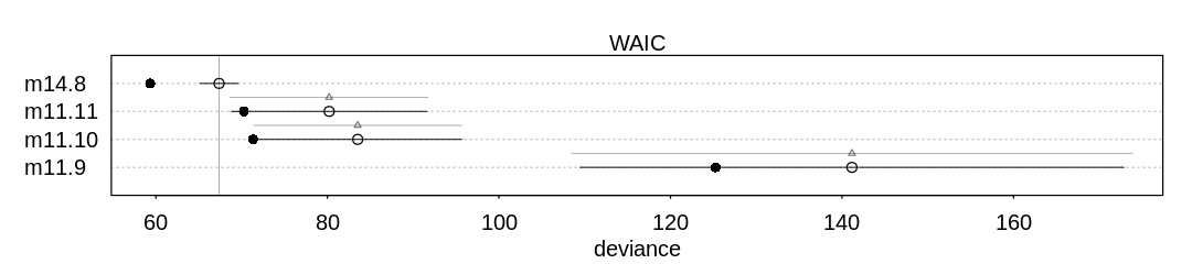
Raw data (preceding plot):
       WAIC      SE       dWAIC    dSE      pWAIC    weight
m14.8   67.37541  2.22661  0.00000       NA 4.011871 9.980596e-01
m11.11  80.20808 11.40787 12.83267 11.55343 4.972381 1.631467e-03
m11.10  83.53601 12.13926 16.16060 12.13169 6.100473 3.089778e-04
m11.9  141.15520 31.71029 73.77979 32.71638 7.945491 9.507763e-17
The new model does better overall relative to m11.1 because it presumably has a more accurate
method of estimating the contact between islands. See the first section of 14.5.1 for how the
new model improves upon the old low/high contact indicator.
The new model also has the lowest penalty term (effective number of parameters). Notice in the
precis output above it has 10 intercept terms, and 5 other terms. This is much more than the 5
parameters in m11.1, also above. It achieves this relative to m11.1 because of the significant
regularization provided by parameter sharing.
14M5. Modify the phylogenetic distance example to use group size as the outcome and brain size as a predictor. Assuming brain size influences group size, what is your estimate of the effect? How does phylogeny influence the estimate?
Answer. First, let’s reproduce the results from the chapter:
data(Primates301)
data(Primates301_nex)

d <- Primates301
d$name <- as.character(d$name)
dstan <- d[complete.cases(d$group_size, d$body, d$brain), ]
spp_obs <- dstan$name

dat_list <- list(
  N_spp = nrow(dstan),
  M = standardize(log(dstan$body)),
  B = standardize(log(dstan$brain)),
  G = standardize(log(dstan$group_size)),
  Imat = diag(nrow(dstan))
)
m14.9 <- ulam(
  alist(
    B ~ multi_normal(mu, SIGMA),
    mu <- a + bM * M + bG * G,
    matrix[N_spp, N_spp]:SIGMA <- Imat * sigma_sq,
    a ~ normal(0, 1),
    c(bM, bG) ~ normal(0, 0.5),
    sigma_sq ~ exponential(1)
  ),
  data = dat_list, chains = 4, cores = 4
)
display(precis(m14.9, depth=2), mimetypes="text/plain")

library(ape)
tree_trimmed <- keep.tip(Primates301_nex, spp_obs)
Rbm <- corBrownian(phy = tree_trimmed)
V <- vcv(Rbm)

# put species in right order
dat_list$V <- V[spp_obs, spp_obs]
# convert to correlation matrix
dat_list$R <- dat_list$V / max(V)

m14.10 <- ulam(
  alist(
    B ~ multi_normal(mu, SIGMA),
    mu <- a + bM * M + bG * G,
    matrix[N_spp, N_spp]:SIGMA <- R * sigma_sq,
    a ~ normal(0, 1),
    c(bM, bG) ~ normal(0, 0.5),
    sigma_sq ~ exponential(1)
  ),
  data = dat_list, chains = 4, cores = 4
)
display(precis(m14.10, depth=2), mimetypes="text/plain")

Dmat <- cophenetic(tree_trimmed)
# add scaled and reordered distance matrix
dat_list$Dmat <- Dmat[spp_obs, spp_obs] / max(Dmat)

m14.11 <- ulam(
  alist(
    B ~ multi_normal(mu, SIGMA),
    mu <- a + bM * M + bG * G,
    matrix[N_spp, N_spp]:SIGMA <- cov_GPL1(Dmat, etasq, rhosq, 0.01),
    a ~ normal(0, 1),
    c(bM, bG) ~ normal(0, 0.5),
    etasq ~ half_normal(1, 0.25),
    rhosq ~ half_normal(3, 0.25)
  ),
  data = dat_list, chains = 4, cores = 4
)
display(precis(m14.11, depth=2), mimetypes="text/plain")
         mean          sd          5.5%        94.5%      n_eff    Rhat4
a        -0.0001731167 0.017310086 -0.02790983 0.02609835 1939.636 0.9986765
bG        0.1230980344 0.023572481  0.08502910 0.16036884 1088.188 1.0011412
bM        0.8930430495 0.023047869  0.85791614 0.93003799 1069.554 1.0030455
sigma_sq  0.0473859234 0.005699073  0.03923401 0.05715970 1300.850 1.0026744
Warning message in Initialize.corPhyl(phy, dummy.df):
“No covariate specified, species will be taken as ordered in the data frame. To avoid this message, specify a covariate containing the species names with the 'form' argument.”
         mean        sd         5.5%        94.5%      n_eff    Rhat4
a        -0.18873820 0.16496198 -0.44557098 0.07618946 2216.384 1.0027970
bG       -0.01217738 0.01971775 -0.04277674 0.01980523 2350.256 0.9990575
bM        0.70105765 0.03861462  0.63972330 0.76345226 1776.208 1.0010190
sigma_sq  0.16148768 0.01875378  0.13339710 0.19432609 2409.753 1.0005959
      mean        sd          5.5%        94.5%      n_eff    Rhat4
a     -0.06587284 0.076292599 -0.18646383 0.05812055 2012.089 0.9999619
bG     0.04981556 0.023797105  0.01034797 0.08758256 2213.185 1.0003827
bM     0.83321792 0.030898044  0.78324467 0.88101712 2727.300 0.9988425
etasq  0.03494790 0.006854313  0.02494174 0.04695430 1937.816 0.9993151
rhosq  2.79131896 0.250754096  2.39426624 3.20118552 2170.700 0.9996398
Reversing the prediction problem:
dat_list <- list(
  N_spp = nrow(dstan),
  M = standardize(log(dstan$body)),
  B = standardize(log(dstan$brain)),
  G = standardize(log(dstan$group_size)),
  Imat = diag(nrow(dstan))
)
m14.9_reversed <- ulam(
  alist(
    G ~ multi_normal(mu, SIGMA),
    mu <- a + bM * M + bB * B,
    matrix[N_spp, N_spp]:SIGMA <- Imat * sigma_sq,
    a ~ normal(0, 1),
    c(bM, bB) ~ normal(0, 0.5),
    sigma_sq ~ exponential(1)
  ),
  data = dat_list, chains = 4, cores = 4
)
display(precis(m14.9_reversed, depth=2), mimetypes="text/plain")

# put species in right order
dat_list$V <- V[spp_obs, spp_obs]
# convert to correlation matrix
dat_list$R <- dat_list$V / max(V)

m14.10_reversed <- ulam(
  alist(
    G ~ multi_normal(mu, SIGMA),
    mu <- a + bM * M + bB * B,
    matrix[N_spp, N_spp]:SIGMA <- R * sigma_sq,
    a ~ normal(0, 1),
    c(bM, bB) ~ normal(0, 0.5),
    sigma_sq ~ exponential(1)
  ),
  data = dat_list, chains = 4, cores = 4
)
display(precis(m14.10_reversed, depth=2), mimetypes="text/plain")

# add scaled and reordered distance matrix
dat_list$Dmat <- Dmat[spp_obs, spp_obs] / max(Dmat)

m14.11_reversed <- ulam(
  alist(
    G ~ multi_normal(mu, SIGMA),
    mu <- a + bM * M + bB * B,
    matrix[N_spp, N_spp]:SIGMA <- cov_GPL1(Dmat, etasq, rhosq, 0.01),
    a ~ normal(0, 1),
    c(bM, bB) ~ normal(0, 0.5),
    etasq ~ half_normal(1, 0.25),
    rhosq ~ half_normal(3, 0.25)
  ),
  data = dat_list, chains = 4, cores = 4
)
display(precis(m14.11_reversed, depth=2), mimetypes="text/plain")
         mean         sd         5.5%        94.5%       n_eff     Rhat4
a        -0.001417642 0.05685219 -0.09147605  0.08793679 1327.7488 0.9992159
bB        1.004936856 0.20442226  0.68104136  1.34138179  854.5307 1.0005631
bM       -0.337334331 0.20456292 -0.67326748 -0.01079579  828.9535 1.0016998
sigma_sq  0.519471576 0.06055068  0.42832399  0.61695123 1429.3501 1.0018326
         mean        sd        5.5%         94.5%     n_eff    Rhat4
a        -0.47774105 0.5678362 -1.359264822 0.4414133 1496.797 1.000575
bB       -0.07150671 0.2583164 -0.476816067 0.3477977 1091.952 1.000832
bM        0.34676958 0.2160707  0.001476129 0.6938241 1003.165 1.001472
sigma_sq  2.68982107 0.3120843  2.234004692 3.2161848 1479.938 1.003012
      mean       sd        5.5%       94.5%      n_eff     Rhat4
a     -0.5021950 0.3442075 -1.0440793 0.03602275 1511.5889 1.000513
bB     0.1850170 0.2626387 -0.2375381 0.60738516  968.2030 1.000422
bM     0.1880509 0.2259942 -0.1873261 0.54406083  989.1999 1.000826
etasq  0.9309690 0.1206105  0.7537561 1.14232420 1593.3978 1.000191
rhosq  3.0219251 0.2384142  2.6610231 3.40037960 1592.1098 1.003639
Interestingly, the ordinary regression model makes an even more extreme prediction about how group size influences brain size than the reverse. Still, the uncertainties are large.
The addition of phylogeny once again removes the presumed effect. The uncertainties are so large in these latter two models that they really say almost nothing about an association.
14H1. Let’s revisit the Bangladesh fertility data, data(bangladesh), from the practice
problems for Chapter 13. Fit a model with both varying intercepts by district_id and varying
slopes of urban by district_id. You are still predicting use.contraception. Inspect the
correlation between the intercepts and slopes. Can you interpret this correlation, in terms of what
it tells you about the pattern of contraceptive use in the sample? It might help to plot the mean
(or median) varying effect estimates for both the intercepts and slopes, by district. Then you can
visualize the correlation and maybe more easily think through what it means to have a particular
correlation. Plotting predicted proportion of women using contraception, with urban women on one
axis and rural on the other, might also help.
Answer. To review, the help for the bangladesh data.frame:
data(bangladesh)
display(help(bangladesh))

bc_df <- bangladesh
bc_df$district_id <- as.integer(as.factor(bc_df$district))
| bangladesh {rethinking} | R Documentation |
Bangladesh contraceptive use data
Description
Contraceptive use data from 1934 Bangladeshi women.
Usage
data(bangladesh)
Format
woman : ID number for each woman in sample
district : Number for each district
use.contraception : 0/1 indicator of contraceptive use
living.children : Number of living children
age.centered : Centered age
urban : 0/1 indicator of urban context
References
Bangladesh Fertility Survey, 1989
A head and summary of the bangladesh data.frame, with the new variable suggested by the author
in question 13H1:
display(head(bc_df))
display(summary(bc_df))
| woman | district | use.contraception | living.children | age.centered | urban | district_id | |
|---|---|---|---|---|---|---|---|
| <int> | <int> | <int> | <int> | <dbl> | <int> | <int> | |
| 1 | 1 | 1 | 0 | 4 | 18.4400 | 1 | 1 |
| 2 | 2 | 1 | 0 | 1 | -5.5599 | 1 | 1 |
| 3 | 3 | 1 | 0 | 3 | 1.4400 | 1 | 1 |
| 4 | 4 | 1 | 0 | 4 | 8.4400 | 1 | 1 |
| 5 | 5 | 1 | 0 | 1 | -13.5590 | 1 | 1 |
| 6 | 6 | 1 | 0 | 1 | -11.5600 | 1 | 1 |
     woman           district     use.contraception living.children
 Min.   :   1.0   Min.   : 1.00   Min.   :0.0000    Min.   :1.000
 1st Qu.: 484.2   1st Qu.:14.00   1st Qu.:0.0000    1st Qu.:1.000
 Median : 967.5   Median :29.00   Median :0.0000    Median :3.000
 Mean   : 967.5   Mean   :29.35   Mean   :0.3925    Mean   :2.652
 3rd Qu.:1450.8   3rd Qu.:45.00   3rd Qu.:1.0000    3rd Qu.:4.000
 Max.   :1934.0   Max.   :61.00   Max.   :1.0000    Max.   :4.000
  age.centered            urban         district_id
 Min.   :-13.560000   Min.   :0.0000   Min.   : 1.00
 1st Qu.: -7.559900   1st Qu.:0.0000   1st Qu.:14.00
 Median : -1.559900   Median :0.0000   Median :29.00
 Mean   :  0.002198   Mean   :0.2906   Mean   :29.25
 3rd Qu.:  6.440000   3rd Qu.:1.0000   3rd Qu.:45.00
 Max.   : 19.440000   Max.   :1.0000   Max.   :60.00
Sampling from the varying intercepts model:
# If you want to reproduce results from the previous chapter:
#
# bc_dat <- list(
# UseContraception = bc_df$use.contraception,
# DistrictId = bc_df$district_id
# )
# m_bc_ve <- ulam(
# alist(
# UseContraception ~ dbinom(1, p),
# logit(p) <- a[DistrictId],
# a[DistrictId] ~ dnorm(a_bar, sigma),
# a_bar ~ dnorm(0, 1.5),
# sigma ~ dexp(1)
# ),
# data = bc_dat, chains = 4, cores = 4, log_lik = TRUE
# )
bc_dat <- list(
UseContraception = bc_df$use.contraception,
DistrictId = bc_df$district_id,
Urban = bc_df$urban
)
m_bc_vis <- ulam(
alist(
UseContraception ~ dbinom(1, p),
logit(p) <- a_district[DistrictId] + b_district[DistrictId] * Urban,
c(a_district, b_district)[DistrictId] ~ multi_normal(c(a, b), Rho, sigma_intercepts_slopes),
a ~ normal(0, 2),
b ~ normal(0, 0.5),
sigma_intercepts_slopes ~ exponential(1),
Rho ~ lkj_corr(2)
),
data = bc_dat, chains = 4, cores = 4, log_lik = TRUE
)
display(precis(m_bc_vis, depth=3), mimetypes="text/plain")
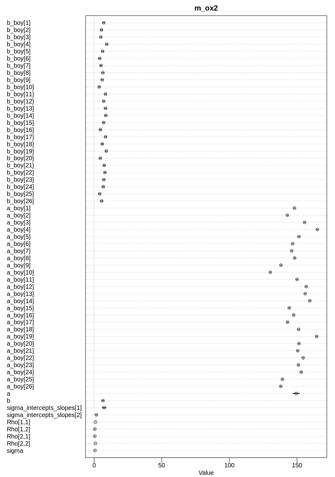
iplot(function() {
plot(precis(m_bc_vis, depth=3), main="m_bc_vis")
}, ar=0.4)
post <- extract.samples(m_bc_vis) # posterior
R <- rlkjcorr(1e4, K = 2, eta = 2) # prior
iplot(function() {
dens(post$Rho[, 1, 2], xlim = c(-1, 1))
dens(R[, 1, 2], add = TRUE, lty = 2)
})
Warning message:
“Bulk Effective Samples Size (ESS) is too low, indicating posterior means and medians may be unreliable.
Running the chains for more iterations may help. See
https://mc-stan.org/misc/warnings.html#bulk-ess”
Warning message:
“Tail Effective Samples Size (ESS) is too low, indicating posterior variances and tail quantiles may be unreliable.
Running the chains for more iterations may help. See
https://mc-stan.org/misc/warnings.html#tail-ess”
                           mean        sd           5.5%          94.5%
b_district[1]               1.0670860  0.3782827     0.4859153953 1.6648881
b_district[2]               0.5967072  0.6645532    -0.4330004363 1.6322922
b_district[3]               0.8848223  0.8057362    -0.3856858371 2.2487559
b_district[4]               1.5814457  0.6347096     0.6560098348 2.6659842
b_district[5]               0.6113797  0.5942621    -0.3188659912 1.5578244
b_district[6]               1.2810511  0.5527699     0.4667433362 2.2225933
b_district[7]               0.7745289  0.6689434    -0.2951438126 1.8745062
b_district[8]               0.9065896  0.6014774     0.0002929298 1.8780210
b_district[9]               0.9863604  0.6166353     0.0425672943 1.9837517
b_district[10]              1.1954027  0.7592615     0.0276866328 2.4434961
b_district[11]              1.5756218  0.8116946     0.4444062308 2.9595681
b_district[12]              0.4322015  0.5665931    -0.4999139671 1.3354042
b_district[13]              0.2684581  0.5874672    -0.6925710533 1.2110490
b_district[14]              1.2110843  0.4319248     0.5424204957 1.9125391
b_district[15]              0.4493872  0.5861374    -0.4998182743 1.3609454
b_district[16]              0.5669155  0.6321994    -0.4256460915 1.5818233
b_district[17]              0.7624304  0.6745130    -0.3045817881 1.8874580
b_district[18]              0.8479431  0.4911165     0.0857845437 1.6496457
b_district[19]              0.9680160  0.6254921     0.0303852148 2.0321759
b_district[20]              0.5403988  0.6952316    -0.5619983408 1.6191578
b_district[21]             -0.3209662  0.6859289    -1.4403290374 0.7075015
b_district[22]              0.9749350  0.6772639    -0.0584712608 2.1394007
b_district[23]              0.8028469  0.6992094    -0.2879172061 1.9132030
b_district[24]              1.2329838  0.7372550     0.1094543016 2.4527721
b_district[25]              0.1879679  0.4248847    -0.5040083386 0.8567129
b_district[26]              0.5668825  0.7233731    -0.5650370280 1.7357724
b_district[27]              1.1476359  0.6180868     0.2054302074 2.1557858
b_district[28]              0.7334328  0.6005227    -0.2234647593 1.6730947
b_district[29]              1.1410977  0.5579254     0.2976138234 2.0465502
b_district[30]              1.0106844  0.5002790     0.2772004374 1.8338426
⋮                          ⋮           ⋮            ⋮             ⋮
a_district[39]             -0.24878952 3.446544e-01 -0.8001652     0.30037495
a_district[40]             -0.53367224 4.056508e-01 -1.1726077     0.11575554
a_district[41]             -0.08785561 3.647116e-01 -0.6613238     0.48234779
a_district[42]             -0.05918072 5.055008e-01 -0.8316718     0.77688896
a_district[43]             -0.22036656 3.018605e-01 -0.6984655     0.24937437
a_district[44]             -1.05308364 3.537547e-01 -1.6495761    -0.50317067
a_district[45]             -0.91672877 3.193301e-01 -1.4355843    -0.41527769
a_district[46]             -0.09571376 2.228935e-01 -0.4450982     0.26582506
a_district[47]             -0.51778990 4.465133e-01 -1.2312732     0.21138532
a_district[48]             -0.22569530 3.243286e-01 -0.7331933     0.30002079
a_district[49]             -1.04824482 5.298423e-01 -1.9150630    -0.27016833
a_district[50]             -0.67188490 4.024037e-01 -1.3064462    -0.02679504
a_district[51]             -0.64603156 3.617746e-01 -1.2429197    -0.06510586
a_district[52]             -0.11721394 2.784987e-01 -0.5601760     0.32948042
a_district[53]             -0.70873036 5.682276e-01 -1.5958060     0.20074087
a_district[54]             -0.75671498 6.164120e-01 -1.7673297     0.23632531
a_district[55]             -0.10909625 3.251141e-01 -0.6168951     0.42430576
a_district[56]             -1.17789470 3.753756e-01 -1.7906242    -0.60817455
a_district[57]             -0.17468722 3.562620e-01 -0.7293605     0.39079686
a_district[58]             -1.17842367 4.955465e-01 -2.0236499    -0.42535810
a_district[59]             -1.15104807 3.848318e-01 -1.7852631    -0.56316102
a_district[60]             -1.17134926 3.309090e-01 -1.7302584    -0.68202729
a                          -0.68697115 9.680213e-02 -0.8431896    -0.53422309
b                           0.64241389 1.533845e-01  0.3911194     0.89095418
sigma_intercepts_slopes[1]  0.57516450 9.473592e-02  0.4356859     0.73634803
sigma_intercepts_slopes[2]  0.76059552 1.976562e-01  0.4589757     1.08665688
Rho[1,1]                    1.00000000 0.000000e+00  1.0000000     1.00000000
Rho[1,2]                   -0.65363331 1.671887e-01 -0.8613258    -0.34409840
Rho[2,1]                   -0.65363331 1.671887e-01 -0.8613258    -0.34409840
Rho[2,2]                    1.00000000 6.272117e-17  1.0000000     1.00000000
                           n_eff     Rhat4
b_district[1]              1831.8290 1.0012389
b_district[2]              2883.8034 0.9994656
b_district[3]              2096.1790 0.9996167
b_district[4]               742.8528 1.0039141
b_district[5]              2158.3104 0.9983583
b_district[6]              1916.0610 0.9987753
b_district[7]              2448.2445 0.9993163
b_district[8]              1779.2636 1.0011896
b_district[9]              2200.3913 0.9991816
b_district[10]             1714.6876 1.0003149
b_district[11]             1021.2957 1.0014837
b_district[12]             3222.1393 1.0006625
b_district[13]             2065.5455 0.9998587
b_district[14]             1408.5814 1.0017142
b_district[15]             2473.9455 0.9988708
b_district[16]             1695.4276 1.0019869
b_district[17]             2690.2394 0.9987431
b_district[18]             2195.1137 0.9999696
b_district[19]             1638.6104 1.0022221
b_district[20]             2519.0662 0.9989753
b_district[21]              921.4559 1.0005069
b_district[22]             2082.2386 1.0003840
b_district[23]             2111.5169 1.0019826
b_district[24]             1380.2483 1.0008525
b_district[25]             1650.5842 1.0014639
b_district[26]             2522.6748 1.0012108
b_district[27]             1632.7972 1.0001834
b_district[28]             3012.6085 0.9992483
b_district[29]             1858.0194 0.9996650
b_district[30]             1301.2451 1.0008541
⋮                          ⋮         ⋮
a_district[39]             2481.3080 1.0003322
a_district[40]             1950.4880 1.0025755
a_district[41]             2499.2493 0.9988345
a_district[42]             1573.8640 1.0001231
a_district[43]             2089.1375 0.9988561
a_district[44]             2712.3422 0.9987354
a_district[45]             2734.5355 1.0001725
a_district[46]             2624.5404 0.9995971
a_district[47]             2193.7884 0.9993473
a_district[48]             1930.0847 0.9995102
a_district[49]             2290.7133 0.9989410
a_district[50]             2363.4590 0.9991670
a_district[51]             2288.5704 0.9997117
a_district[52]             1992.2301 0.9997977
a_district[53]             2065.2941 0.9997024
a_district[54]             1532.5275 0.9999255
a_district[55]             2246.6413 0.9994746
a_district[56]             2510.3441 0.9997795
a_district[57]             1348.0636 0.9997778
a_district[58]             2411.5027 0.9985544
a_district[59]             2692.0315 0.9991757
a_district[60]             2315.3140 0.9989207
a                          1699.3030 0.9988051
b                          1236.1160 1.0003488
sigma_intercepts_slopes[1]  604.1727 1.0028934
sigma_intercepts_slopes[2]  263.0453 1.0080110
Rho[1,1]                         NaN       NaN
Rho[1,2]                    379.9839 1.0097282
Rho[2,1]                    379.9839 1.0097282
Rho[2,2]                   1937.6490 0.9979980
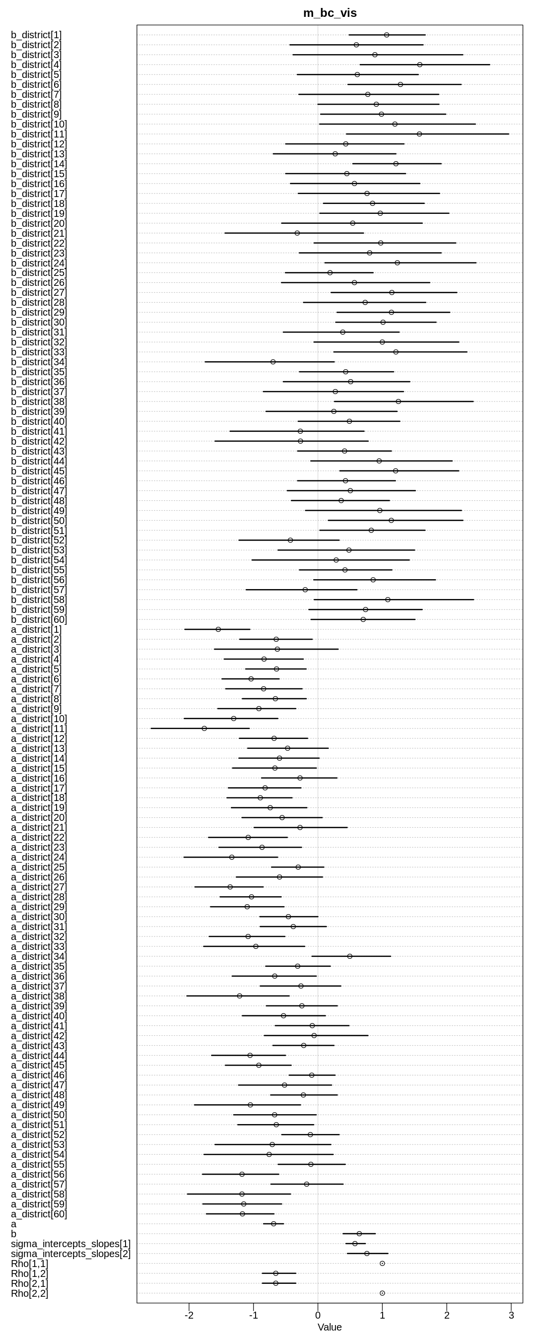
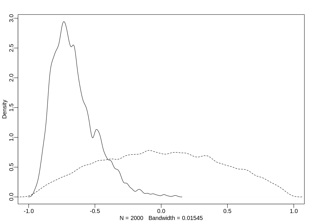
Not surprisingly, the b slope parameter and most of the b_district are positive. Normally,
living in an urban area makes one more open to ideas like contraception. The a parameters are
likely negative because in general many women do not use contraception.
The correlation is negative, because a is typically negative and b is typically positive. It is
also relatively large in absolute magnitude, implying that a more negative intercept is associated
with a more positive slope (and vice versa). We can see this in a plot of mean intercepts vs. mean
slopes:
iplot(function() {
  post <- extract.samples(m_bc_vis)
  a2 <- apply(post$a_district, 2, mean)
  b2 <- apply(post$b_district, 2, mean)

  plot(a2, b2,
    xlab = "intercept", ylab = "slope",
    pch = 1, col = rangi2, ylim = c(min(b2) - 0.1, max(b2) + 0.1),
    xlim = c(min(a2) - 0.1, max(a2) + 0.1)
  )

  Mu_est <- c(mean(post$a), mean(post$b))
  rho_est <- mean(post$Rho[, 1, 2])
  sa_est <- mean(post$sigma_intercepts_slopes[, 1])
  sb_est <- mean(post$sigma_intercepts_slopes[, 2])
  cov_ab <- sa_est * sb_est * rho_est
  Sigma_est <- matrix(c(sa_est^2, cov_ab, cov_ab, sb_est^2), ncol = 2)
  library(ellipse)
  for (l in c(0.1, 0.3, 0.5, 0.8, 0.99)) {
    lines(ellipse(Sigma_est, centre = Mu_est, level = l),
      col = col.alpha("black", 0.2)
    )
  }
})
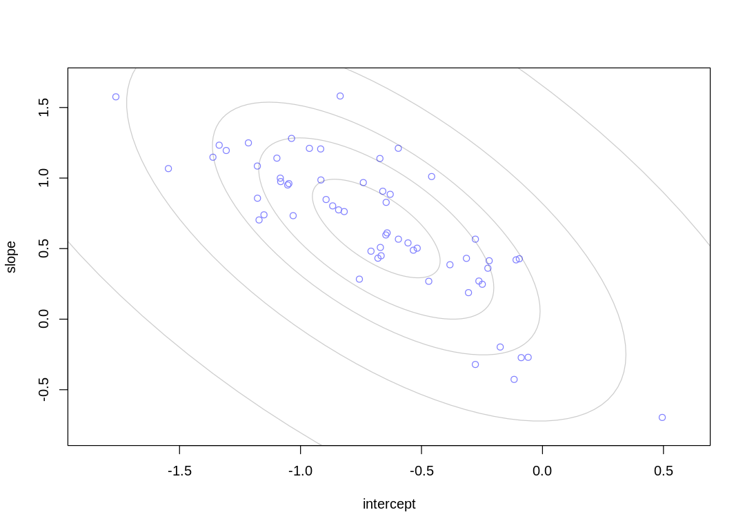
This is a similar relationship to what we saw in the cafe example at the start of the chapter; more extreme intercepts (cafes, districts) are associated with more extreme slopes. In this case the districts with especially low contraceptive use are associated with a greater increase in use when a woman ‘moves’ to an urban area within the district.
14H2. Now consider the predictor variables age.centered and living.children, also contained
in data(bangladesh). Suppose that age influences contraceptive use (changing attitudes) and number
of children (older people have had more time to have kids). Number of children may also directly
influence contraceptive use. Draw a DAG that reflects these hypothetical relationships. Then build
models needed to evaluate the DAG. You will need at least two models. Retain district and urban,
as in 14H1. What do you conclude about the causal influence of age and children?
Answer. [cc]: https://en.wikipedia.org/wiki/Counterfactual_conditional
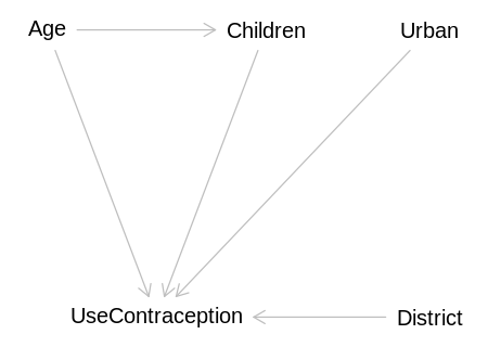
Consider the following causal diagram. Is this diagram reasonable? The author asked us to only consider this one DAG, but it’s worth thinking whether it’s reasonable so we know what to expect from our inferences.
The Age variable only has arrows pointing out of it. As discussed elsewhere (see question 12H7),
this is the only way we should put time-based variables on DAGs. We can think about Age as
describing the timing of someone’s birth. In terms of a [counterfactual conditional][cc], we would
say that if a woman had been born e.g. 10 years earlier she would not have used contraception. A
counterfactual conditional like this describes a causal theory, but expressed regarding the past.
Casual theories should still be tested, when possible, by actively controlling a variable in the
future. In this case we won’t be able to test the theory in the future (as well as the past) because
we can’t control the date of anyone’s birth, unless we ran an experiment with identical twins where
we somehow froze the zygote of one twin in time for years. We’ll include a description of all
existing and potential arrows in this DAG as counterfactual conditionals below.
It’s reasonable to think that Age could affect Urban. More people are moving to cities every
year across the world, for jobs, and so in general we’d expect younger women to be living in cities.
That is, if a woman was born later she would be more likely to be urban.
It’s possible that Age could affect District if there was a people migration happening across
the country at one point in the past and slightly older women were less likely to move. That is, if
a woman was born later she could be living in a different district.
Some districts could be more urbanized and therefore District could predict Urban, and vice
versa. That is, if a woman was living in a different district she could be more likely to be urban.
If a woman was not in an urban area she would be more likely to be in a different district.
Some districts might have governmental programs or tax incentives to encourage or discourage
children, implying a relationship between District and Children mediated by the program. This
would confound our causal inference about the effect of Children on UseContraception if we
didn’t include District in our model. Similarly, for urban programs encouraging or discouraging
children. If a woman was living in a different district, she may have had more or fewer children.
It’s also likely that women move to more rural areas for e.g. cheaper housing when they have more children, or to districts with cheaper housing and costs of living. That is, a woman had fewer children, she may be living in a less urban area or in general somewhere else.
Like the controversy over global warming in the United States, there are often many possible confounds we can suggest to make a DAG more complicated. It can be hard to decide which need to be included in every model without getting into a lot of details.
In this question we are predicting UseContraception from Children but we’d typically think of
the opposite causal path: contraception clearly influences the number of children a woman will have.
In this case, we are essentially assuming that the number of children a woman has in the present
influences her present decision to use contraception. In general, though, these variables interact,
so we have to look at the casual paths similar as a causal time series similar to how the author
treated the causal influence of group size on brain size at the beginning of section 14.5.2. Our
causal inferences here will only apply to the point in time when these surveys were taken.
We’ll ignore all of this. The DAG expected by the question:
library(dagitty)

expected_dag <- dagitty('
dag {
    bb="0,0,1,1"
    Age [pos="0.3,0.1"]
    Children [exposure,pos="0.5,0.1"]
    District [pos="0.65,0.2"]
    Urban [pos="0.65,0.1"]
    UseContraception [outcome,pos="0.4,0.2"]
    Age -> Children
    Age -> UseContraception
    Children -> UseContraception
    District -> UseContraception
    Urban -> UseContraception
}')
iplot(function() plot(expected_dag), scale=10)
Attaching package: ‘dagitty’
The following object is masked from ‘package:ape’:

    edges
Implied conditional independencies:
display(impliedConditionalIndependencies(expected_dag))
Age _||_ Dstr
Age _||_ Urbn
Chld _||_ Dstr
Chld _||_ Urbn
Dstr _||_ Urbn
We will build two models, as the question suggests. The first will include both predictors, so we
can infer the direct/total causal effect of children on UseContraception:
display(adjustmentSets(expected_dag, exposure="Children", outcome="UseContraception", effect="direct"))
display(adjustmentSets(expected_dag, exposure="Children", outcome="UseContraception", effect="total"))
{ Age }
{ Age }
The first model will also predict the direct effect of Age on UseContraception:
display(adjustmentSets(expected_dag, exposure="Age", outcome="UseContraception", effect="direct"))
{ Children }
The second will include only Age so we can infer the total causal effect of Age on
UseContraception:
display(adjustmentSets(expected_dag, exposure="Age", outcome="UseContraception", effect="total"))
{}
Fitting the first model:
data(bangladesh)
bc_df <- bangladesh
bc_df$district_id <- as.integer(as.factor(bc_df$district))

bc_dat <- list(
  UseContraception = bc_df$use.contraception,
  DistrictId = bc_df$district_id,
  Urban = bc_df$urban,
  Age = standardize(bc_df$age.centered),
  Children = bc_df$living.children
)
m_bc_age_children <- ulam(
  alist(
    UseContraception ~ dbinom(1, p),
    logit(p) <- a_district[DistrictId] + b_district[DistrictId] * Urban + bAge * Age +
a_children[Children],
    c(a_district, b_district)[DistrictId] ~ multi_normal(c(a, b), Rho, sigma_intercepts_slopes),
    a_children[Children] ~ normal(0, 1),
    a ~ normal(0, 2),
    b ~ normal(0, 0.5),
    bAge ~ normal(0, 0.5),
    sigma_intercepts_slopes ~ exponential(1),
    Rho ~ lkj_corr(2)
  ),
  data = bc_dat, chains = 4, cores = 4, log_lik = TRUE
)
display(precis(m_bc_age_children, depth=3), mimetypes="text/plain")
iplot(function() {
  plot(precis(m_bc_age_children, depth=3), main="m_bc_age_children")
}, ar=0.4)
Warning message:
“The largest R-hat is NA, indicating chains have not mixed.
Running the chains for more iterations may help. See
https://mc-stan.org/misc/warnings.html#r-hat”
Warning message:
“Bulk Effective Samples Size (ESS) is too low, indicating posterior means and medians may be unreliable.
Running the chains for more iterations may help. See
https://mc-stan.org/misc/warnings.html#bulk-ess”
Warning message:
“Tail Effective Samples Size (ESS) is too low, indicating posterior variances and tail quantiles may be unreliable.
Running the chains for more iterations may help. See
https://mc-stan.org/misc/warnings.html#tail-ess”
                           mean        sd           5.5%        94.5%
b_district[1]               1.0999167  0.3908649     0.49159563 1.7417916
b_district[2]               0.7624000  0.6713341    -0.29147820 1.8229521
b_district[3]               1.0043785  0.8060123    -0.20528392 2.3405111
b_district[4]               1.6438375  0.6611769     0.66845155 2.7468812
b_district[5]               0.7022189  0.5919901    -0.23480486 1.6426724
b_district[6]               1.4202445  0.5546021     0.60059064 2.3576044
b_district[7]               0.9034358  0.7198666    -0.18233987 2.0596096
b_district[8]               1.0075832  0.6370145     0.03735138 2.0919893
b_district[9]               1.1294339  0.6425540     0.14775703 2.1998940
b_district[10]              1.1811700  0.7393612     0.05655746 2.3937003
b_district[11]              1.5655565  0.8298174     0.33789497 2.9904372
b_district[12]              0.4899962  0.5848951    -0.46789684 1.3872553
b_district[13]              0.3906549  0.5638410    -0.54148595 1.2365869
b_district[14]              1.4123033  0.4611426     0.69587260 2.1682716
b_district[15]              0.4825745  0.6121071    -0.52356196 1.4521823
b_district[16]              0.5243952  0.6783461    -0.53337786 1.6515876
b_district[17]              0.8794557  0.7167730    -0.23753859 2.0253755
b_district[18]              1.0268427  0.5122685     0.21549225 1.8279752
b_district[19]              1.0270314  0.6237950     0.06036288 2.0466071
b_district[20]              0.5158529  0.7126419    -0.66672066 1.6332599
b_district[21]             -0.3279448  0.7220129    -1.58727814 0.7005328
b_district[22]              1.1335031  0.7273222    -0.00905651 2.3106420
b_district[23]              0.9190812  0.7432049    -0.20580069 2.0794233
b_district[24]              1.2563269  0.7596747     0.09519452 2.4983379
b_district[25]              0.4333071  0.4399538    -0.26694340 1.1220195
b_district[26]              0.7074407  0.7235723    -0.42221307 1.8767707
b_district[27]              1.1893079  0.5969365     0.25626517 2.1375584
b_district[28]              0.7021765  0.6034404    -0.30269080 1.6450539
b_district[29]              1.2046125  0.5733478     0.32493704 2.1606517
b_district[30]              0.9428385  0.4741211     0.22253355 1.7132574
⋮                          ⋮           ⋮            ⋮           ⋮
a_district[44]             -1.00757529 6.136324e-01 -1.9911938  -0.02934434
a_district[45]             -0.97830892 5.980057e-01 -1.9538494  -0.02719440
a_district[46]             -0.03314476 5.566992e-01 -0.9117773   0.86163084
a_district[47]             -0.38205712 6.907393e-01 -1.4876866   0.73290678
a_district[48]             -0.10582759 6.133921e-01 -1.0728309   0.85300833
a_district[49]             -0.94369673 7.508873e-01 -2.1100061   0.23350557
a_district[50]             -0.51192605 6.692862e-01 -1.5518202   0.56943445
a_district[51]             -0.67770025 6.343153e-01 -1.6873408   0.33168960
a_district[52]             -0.06297412 5.825162e-01 -0.9578809   0.84667572
a_district[53]             -0.66126462 8.167981e-01 -1.9708303   0.71126875
a_district[54]             -0.70715221 8.193827e-01 -2.0321862   0.58303659
a_district[55]              0.04195840 6.380596e-01 -0.9442829   1.07382583
a_district[56]             -1.11721014 6.541691e-01 -2.1445767  -0.07994060
a_district[57]             -0.01447033 6.520955e-01 -1.0314944   1.03048964
a_district[58]             -1.21266444 6.882528e-01 -2.2795963  -0.09667581
a_district[59]             -1.08185653 6.427204e-01 -2.0945485  -0.07955301
a_district[60]             -1.21806642 6.201448e-01 -2.2460559  -0.27990187
a_children[1]              -1.02952192 5.207069e-01 -1.8500820  -0.19564254
a_children[2]               0.08108856 5.209392e-01 -0.7603851   0.89890579
a_children[3]               0.31428682 5.225278e-01 -0.5115419   1.14501164
a_children[4]               0.29755674 5.199256e-01 -0.5168079   1.12623139
a                          -0.63573454 5.211178e-01 -1.4590586   0.18399513
b                           0.71397519 1.589268e-01  0.4585300   0.96581740
bAge                       -0.22737831 6.922955e-02 -0.3359584  -0.11826217
sigma_intercepts_slopes[1]  0.60466470 1.017295e-01  0.4521114   0.77621481
sigma_intercepts_slopes[2]  0.77828611 2.040382e-01  0.4604246   1.12411203
Rho[1,1]                    1.00000000 0.000000e+00  1.0000000   1.00000000
Rho[1,2]                   -0.64507055 1.684769e-01 -0.8600055  -0.32967889
Rho[2,1]                   -0.64507055 1.684769e-01 -0.8600055  -0.32967889
Rho[2,2]                    1.00000000 6.153016e-17  1.0000000   1.00000000
                           n_eff      Rhat4
b_district[1]              1839.5571  0.9984079
b_district[2]              3409.2984  0.9999534
b_district[3]              1706.9000  0.9987609
b_district[4]               669.9120  1.0055624
b_district[5]              3190.8290  1.0003951
b_district[6]              1044.2280  1.0018416
b_district[7]              2599.6768  1.0010587
b_district[8]              1737.1760  0.9997373
b_district[9]              2613.2646  0.9985529
b_district[10]             1507.0233  1.0003189
b_district[11]             1326.2529  1.0000899
b_district[12]             1944.0288  0.9995990
b_district[13]             2282.0064  0.9993529
b_district[14]             1403.3040  1.0000731
b_district[15]             2218.0897  1.0004139
b_district[16]             2212.6778  1.0010683
b_district[17]             2962.5253  0.9990428
b_district[18]             2344.2862  0.9990850
b_district[19]             2133.9400  0.9998191
b_district[20]             2473.1233  0.9997963
b_district[21]              656.1066  1.0051644
b_district[22]             1823.7037  0.9991960
b_district[23]             2581.8564  0.9991919
b_district[24]             1221.3117  1.0003195
b_district[25]             2773.4273  1.0004201
b_district[26]             2760.2540  0.9990907
b_district[27]             1834.5880  0.9995749
b_district[28]             1917.9901  0.9994573
b_district[29]             1352.9754  0.9996811
b_district[30]             2076.7044  1.0010753
⋮                          ⋮          ⋮
a_district[44]               63.01853 1.0496414
a_district[45]               58.62364 1.0528270
a_district[46]               53.68775 1.0638962
a_district[47]               78.95846 1.0383481
a_district[48]               62.06339 1.0590729
a_district[49]               99.78424 1.0320701
a_district[50]               72.83560 1.0464830
a_district[51]               73.44679 1.0488270
a_district[52]               55.62306 1.0669655
a_district[53]              101.89727 1.0326683
a_district[54]              109.91239 1.0319721
a_district[55]               61.94630 1.0530400
a_district[56]               59.75073 1.0507623
a_district[57]               61.80999 1.0585249
a_district[58]               75.79770 1.0377480
a_district[59]               73.98629 1.0443772
a_district[60]               67.82203 1.0530765
a_children[1]                44.84983 1.0711356
a_children[2]                43.03068 1.0756245
a_children[3]                44.55434 1.0768130
a_children[4]                42.62129 1.0777767
a                            42.14154 1.0779772
b                          1048.78662 1.0006900
bAge                       2819.64745 0.9999493
sigma_intercepts_slopes[1]  695.84499 1.0051581
sigma_intercepts_slopes[2]  210.86961 1.0173553
Rho[1,1]                          NaN       NaN
Rho[1,2]                    489.22550 1.0078223
Rho[2,1]                    489.22550 1.0078223
Rho[2,2]                   1753.63666 0.9979980
Fitting the second model:
bc_dat <- list(
UseContraception = bc_df$use.contraception,
DistrictId = bc_df$district_id,
Urban = bc_df$urban,
Age = standardize(bc_df$age.centered)
)
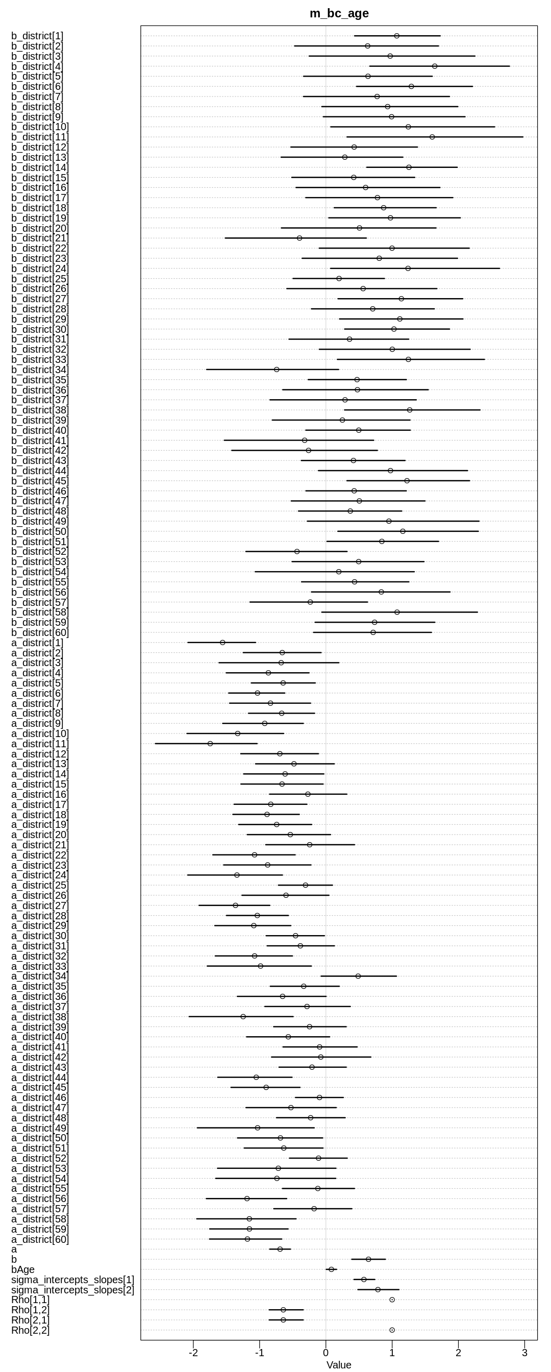
m_bc_age <- ulam(
alist(
UseContraception ~ dbinom(1, p),
logit(p) <- a_district[DistrictId] + b_district[DistrictId] * Urban + bAge * Age,
c(a_district, b_district)[DistrictId] ~ multi_normal(c(a, b), Rho, sigma_intercepts_slopes),
a ~ normal(0, 2),
b ~ normal(0, 0.5),
bAge ~ normal(0, 0.5),
sigma_intercepts_slopes ~ exponential(1),
Rho ~ lkj_corr(2)
),
data = bc_dat, chains = 4, cores = 4, log_lik = TRUE
)
display(precis(m_bc_age, depth=3), mimetypes="text/plain")
iplot(function() {
plot(precis(m_bc_age, depth=3), main="m_bc_age")
}, ar=0.4)
Warning message:
“Bulk Effective Samples Size (ESS) is too low, indicating posterior means and medians may be unreliable.
Running the chains for more iterations may help. See
https://mc-stan.org/misc/warnings.html#bulk-ess”
Warning message:
“Tail Effective Samples Size (ESS) is too low, indicating posterior variances and tail quantiles may be unreliable.
Running the chains for more iterations may help. See
https://mc-stan.org/misc/warnings.html#tail-ess”
                           mean        sd           5.5%         94.5%
b_district[1]               1.0702136  0.4067277     0.43379121  1.7248416
b_district[2]               0.6305582  0.6912087    -0.47099620  1.6988042
b_district[3]               0.9705495  0.7902006    -0.25163575  2.2485909
b_district[4]               1.6429103  0.6505227     0.66302723  2.7696751
b_district[5]               0.6356402  0.6139752    -0.33570188  1.6054755
b_district[6]               1.2899324  0.5596966     0.46314778  2.2128706
b_district[7]               0.7735038  0.7020769    -0.33740407  1.8648556
b_district[8]               0.9321451  0.6491707    -0.06116912  1.9916973
b_district[9]               0.9917004  0.6714883    -0.03799627  2.0999914
b_district[10]              1.2438967  0.7840562     0.07436494  2.5460826
b_district[11]              1.6047628  0.8444329     0.31912278  2.9721018
b_district[12]              0.4267246  0.5973661    -0.52816545  1.3816863
b_district[13]              0.2860661  0.5781811    -0.67536741  1.1610802
b_district[14]              1.2535781  0.4232179     0.61710183  1.9822707
b_district[15]              0.4207730  0.5816601    -0.51392978  1.3405875
b_district[16]              0.5996888  0.6929692    -0.45002673  1.7215217
b_district[17]              0.7783539  0.7053412    -0.30324018  1.9164783
b_district[18]              0.8717355  0.4831137     0.12611949  1.6636872
b_district[19]              0.9747263  0.6338828     0.04406323  2.0289520
b_district[20]              0.5074256  0.7368209    -0.67157506  1.6615544
b_district[21]             -0.3972980  0.6662763    -1.51749499  0.6102074
b_district[22]              0.9984948  0.7441407    -0.10027794  2.1627915
b_district[23]              0.8053357  0.7483680    -0.35752667  1.9867326
b_district[24]              1.2397900  0.7926735     0.07207726  2.6201476
b_district[25]              0.1991053  0.4276917    -0.49510261  0.8834087
b_district[26]              0.5621284  0.7225624    -0.58839125  1.6748054
b_district[27]              1.1391534  0.5962353     0.18383570  2.0653965
b_district[28]              0.7071302  0.5805124    -0.21788665  1.6359116
b_district[29]              1.1159222  0.5861940     0.20646296  2.0684271
b_district[30]              1.0274215  0.5023722     0.28346471  1.8659726
⋮                          ⋮           ⋮            ⋮            ⋮
a_district[40]             -0.56713225 3.942035e-01 -1.196080694  0.05692364
a_district[41]             -0.09445060 3.518192e-01 -0.646965536  0.47154724
a_district[42]             -0.07645624 4.785484e-01 -0.819215319  0.67868498
a_district[43]             -0.20928463 3.245208e-01 -0.706348092  0.30756017
a_district[44]             -1.05076852 3.564967e-01 -1.631410062 -0.51042323
a_district[45]             -0.90137965 3.195985e-01 -1.430802543 -0.39026654
a_district[46]             -0.09572654 2.242291e-01 -0.458310570  0.26297881
a_district[47]             -0.52708188 4.322266e-01 -1.204760880  0.15630742
a_district[48]             -0.23006057 3.313788e-01 -0.745034819  0.29127181
a_district[49]             -1.03023255 5.507298e-01 -1.939590161 -0.17612258
a_district[50]             -0.68555663 3.984149e-01 -1.333323326 -0.04795596
a_district[51]             -0.63496193 3.707027e-01 -1.231812436 -0.04323402
a_district[52]             -0.11045522 2.763375e-01 -0.548731329  0.32194903
a_district[53]             -0.71767053 5.517730e-01 -1.635052142  0.15193477
a_district[54]             -0.73863665 5.836698e-01 -1.661464909  0.14930034
a_district[55]             -0.12110828 3.453037e-01 -0.655014058  0.43152436
a_district[56]             -1.18951735 3.893304e-01 -1.803571667 -0.59085226
a_district[57]             -0.17772950 3.702615e-01 -0.786031845  0.39128593
a_district[58]             -1.15459443 4.728163e-01 -1.948179197 -0.45065063
a_district[59]             -1.15298373 3.783223e-01 -1.753136917 -0.57052335
a_district[60]             -1.18366333 3.435825e-01 -1.755721227 -0.66582234
a                          -0.69088692 9.915224e-02 -0.847275102 -0.53470701
b                           0.64328244 1.582692e-01  0.390786598  0.89773685
bAge                        0.08306864 4.881746e-02  0.006175679  0.16085576
sigma_intercepts_slopes[1]  0.57408849 9.799291e-02  0.424628883  0.73759442
sigma_intercepts_slopes[2]  0.78539789 1.963405e-01  0.483581293  1.10263891
Rho[1,1]                    1.00000000 0.000000e+00  1.000000000  1.00000000
Rho[1,2]                   -0.64207947 1.638724e-01 -0.854575139 -0.34237655
Rho[2,1]                   -0.64207947 1.638724e-01 -0.854575139 -0.34237655
Rho[2,2]                    1.00000000 6.192971e-17  1.000000000  1.00000000
                           n_eff     Rhat4
b_district[1]              1829.9801 1.0010016
b_district[2]              2009.4880 1.0004020
b_district[3]              1741.9526 0.9989266
b_district[4]               743.9184 0.9995581
b_district[5]              2805.5472 0.9998584
b_district[6]              1618.8969 0.9998220
b_district[7]              1825.5960 1.0007015
b_district[8]              1679.4763 0.9997061
b_district[9]              2363.5877 0.9992498
b_district[10]             1563.5257 1.0045377
b_district[11]             1167.8123 1.0002489
b_district[12]             2498.4809 0.9991042
b_district[13]             1756.7462 1.0007052
b_district[14]             1228.6417 1.0001107
b_district[15]             1901.5656 0.9994154
b_district[16]             2039.6668 0.9990231
b_district[17]             2409.0061 0.9997818
b_district[18]             2201.4167 0.9996737
b_district[19]             1558.7646 1.0014130
b_district[20]             1943.8058 1.0000445
b_district[21]              822.0622 1.0015318
b_district[22]             1979.9077 0.9994562
b_district[23]             2290.9894 1.0005602
b_district[24]             1513.2038 0.9984700
b_district[25]             1832.4354 0.9993031
b_district[26]             2059.9716 0.9999822
b_district[27]             1594.2774 1.0006990
b_district[28]             2185.1060 0.9984959
b_district[29]             1720.6701 1.0000656
b_district[30]             1947.2835 0.9995516
⋮                          ⋮         ⋮
a_district[40]             1670.8647 0.9995937
a_district[41]             1792.6930 1.0000349
a_district[42]             1172.3509 0.9993053
a_district[43]             2325.3694 0.9993269
a_district[44]             3272.7154 0.9992261
a_district[45]             2406.2164 0.9993421
a_district[46]             2844.9845 0.9996790
a_district[47]             2090.3225 0.9991635
a_district[48]             2392.3548 1.0011711
a_district[49]             2326.2755 1.0012745
a_district[50]             2666.9974 1.0002669
a_district[51]             2380.2410 0.9985290
a_district[52]             1783.3829 0.9995301
a_district[53]             2138.6105 1.0030239
a_district[54]             1778.1201 0.9996700
a_district[55]             1840.4563 0.9994024
a_district[56]             2513.9127 0.9999035
a_district[57]             1381.4852 1.0009826
a_district[58]             1886.2134 1.0009924
a_district[59]             2061.4345 0.9985233
a_district[60]             1931.9196 1.0007637
a                          1396.8717 1.0008768
b                          1163.2596 1.0003428
bAge                       3897.3416 0.9989784
sigma_intercepts_slopes[1]  645.1497 1.0061509
sigma_intercepts_slopes[2]  240.2612 1.0026197
Rho[1,1]                         NaN       NaN
Rho[1,2]                    442.8782 1.0064511
Rho[2,1]                    442.8782 1.0064511
Rho[2,2]                   1692.5187 0.9979980
In the first model, we see that with more children the likelihood of using birth control goes up, as expected. The likelihood of using birth control also goes down with age, as expected if you assume that younger women are more open to newer ideas like birth control.
In the second model we see the total causal effect of age on whether a woman uses birth control is positive. That is, the older a woman is the more likely she is to use birth control. That is, the tendency for a woman to use birth control as she gets older because she has more children is stronger than the influence of changing acceptance of birth control.
14H3. Modify any models from 14H2 that contained that children variable and model the variable now as a monotonic ordered category, like education from the week we did ordered categories. Education in that example had 8 categories. Children here will have fewer (no one in the sample had 8 children). So modify the code appropriately. What do you conclude about the causal influence of each additional child on use of contraception?
ERROR: The author uses the term week above as if he has a syllabus for the book.
Answer. Fitting the model:
data(bangladesh)
bc_df <- bangladesh
bc_df$district_id <- as.integer(as.factor(bc_df$district))

bc_dat <- list(
  UseContraception = bc_df$use.contraception,
  DistrictId = bc_df$district_id,
  Urban = bc_df$urban,
  Age = standardize(bc_df$age.centered),
  Children = as.integer(bc_df$living.children),
  alpha = rep(2, 3)
)
m_bc_ordered_children <- ulam(
  alist(
    UseContraception ~ dbinom(1, p),
    logit(p) <- bC*sum(delta_j[1:Children]) + a_district[DistrictId] + b_district[DistrictId] *
Urban + bAge * Age,
    c(a_district, b_district)[DistrictId] ~ multi_normal(c(a, b), Rho, sigma_intercepts_slopes),
    bC ~ normal(0, 1),
    a ~ normal(0, 2),
    b ~ normal(0, 0.5),
    bAge ~ normal(0, 0.5),
    sigma_intercepts_slopes ~ exponential(1),
    Rho ~ lkj_corr(2),
    vector[4]: delta_j <<- append_row( 0 , delta ),
    simplex[3]: delta ~ dirichlet( alpha )
  ),
  data = bc_dat, chains = 4, cores = 4, log_lik = TRUE
)
display(precis(m_bc_ordered_children, depth=3), mimetypes="text/plain")
iplot(function() {
  plot(precis(m_bc_ordered_children, depth=3), main="m_bc_ordered_children")
}, ar=0.4)
Warning message:
“Bulk Effective Samples Size (ESS) is too low, indicating posterior means and medians may be unreliable.
Running the chains for more iterations may help. See
https://mc-stan.org/misc/warnings.html#bulk-ess”
Warning message:
“Tail Effective Samples Size (ESS) is too low, indicating posterior variances and tail quantiles may be unreliable.
Running the chains for more iterations may help. See
https://mc-stan.org/misc/warnings.html#tail-ess”
                           mean        sd           5.5%        94.5%
b_district[1]               1.1172469  0.3947964     0.48297366 1.7406465
b_district[2]               0.7614204  0.7128541    -0.32013969 1.8925728
b_district[3]               0.9775367  0.8165073    -0.28479200 2.3091791
b_district[4]               1.6304651  0.6217377     0.70311733 2.6565408
b_district[5]               0.6884590  0.6266713    -0.30505475 1.6964227
b_district[6]               1.3976158  0.5506682     0.58861327 2.3132589
b_district[7]               0.8752725  0.6839709    -0.19915593 1.9709745
b_district[8]               0.9775638  0.6223842     0.02468108 2.0054431
b_district[9]               1.1287229  0.6457095     0.15336211 2.2037115
b_district[10]              1.1993028  0.7611886     0.10176672 2.4951891
b_district[11]              1.5533671  0.8312594     0.32903001 2.9187281
b_district[12]              0.5132767  0.6062558    -0.46498870 1.4522622
b_district[13]              0.3750357  0.5881354    -0.59452498 1.2741826
b_district[14]              1.3850316  0.4405043     0.67993847 2.0776020
b_district[15]              0.4313439  0.6274121    -0.61220327 1.4028669
b_district[16]              0.5163426  0.6432999    -0.46993826 1.5422191
b_district[17]              0.8800332  0.7051507    -0.19434518 1.9770823
b_district[18]              1.0208456  0.4937756     0.23166464 1.8259519
b_district[19]              1.0040505  0.6176643     0.07376052 2.0267407
b_district[20]              0.4920475  0.7194264    -0.65689430 1.6608345
b_district[21]             -0.3435313  0.7086118    -1.55182460 0.6896701
b_district[22]              1.0893223  0.7290794    -0.05315765 2.2403613
b_district[23]              0.8678881  0.7129492    -0.25082946 2.0184497
b_district[24]              1.2810500  0.7522196     0.11836281 2.5333473
b_district[25]              0.4349194  0.4393901    -0.24534788 1.1284563
b_district[26]              0.6664842  0.7000972    -0.46075819 1.7295660
b_district[27]              1.1723796  0.6142847     0.21989934 2.1488261
b_district[28]              0.6975674  0.6067147    -0.28778595 1.6661818
b_district[29]              1.1837080  0.6063302     0.27756238 2.1866475
b_district[30]              0.9411080  0.4801367     0.20010201 1.7490492
⋮                          ⋮           ⋮            ⋮           ⋮
a_district[44]             -2.01565316 3.889580e-01 -2.65596603 -1.4197053
a_district[45]             -1.97231042 3.553071e-01 -2.54360962 -1.4135556
a_district[46]             -1.05993405 2.479984e-01 -1.47103244 -0.6728968
a_district[47]             -1.40711734 4.719714e-01 -2.15791705 -0.6477676
a_district[48]             -1.09022149 3.433844e-01 -1.62885343 -0.5490830
a_district[49]             -1.97443974 5.736895e-01 -2.92491602 -1.0750045
a_district[50]             -1.52572109 4.364849e-01 -2.21756447 -0.8397019
a_district[51]             -1.69507483 3.930730e-01 -2.33437232 -1.0770527
a_district[52]             -1.09322637 3.058946e-01 -1.58148714 -0.5976245
a_district[53]             -1.69162223 6.504140e-01 -2.71149771 -0.6315280
a_district[54]             -1.72704061 6.375521e-01 -2.75649355 -0.7129678
a_district[55]             -0.96697391 3.694604e-01 -1.54392148 -0.3801536
a_district[56]             -2.13901583 4.255826e-01 -2.83738719 -1.4699294
a_district[57]             -1.00697529 3.769271e-01 -1.59853190 -0.4072379
a_district[58]             -2.24133056 5.284252e-01 -3.12622964 -1.4170601
a_district[59]             -2.12211217 4.168315e-01 -2.81841840 -1.4745107
a_district[60]             -2.23019533 3.914657e-01 -2.89008046 -1.6357820
bC                          1.38506932 1.591415e-01  1.13804534  1.6396411
a                          -1.65171232 1.529888e-01 -1.90285604 -1.4009028
b                           0.70576856 1.594368e-01  0.45896996  0.9545962
bAge                       -0.25808498 6.446993e-02 -0.36040392 -0.1548705
sigma_intercepts_slopes[1]  0.60851857 1.033183e-01  0.45612360  0.7832236
sigma_intercepts_slopes[2]  0.77719933 1.977456e-01  0.48570605  1.1170490
Rho[1,1]                    1.00000000 0.000000e+00  1.00000000  1.0000000
Rho[1,2]                   -0.63287420 1.694468e-01 -0.85518047 -0.3378406
Rho[2,1]                   -0.63287420 1.694468e-01 -0.85518047 -0.3378406
Rho[2,2]                    1.00000000 6.513255e-17  1.00000000  1.0000000
delta[1]                    0.73575546 7.864344e-02  0.60302275  0.8571040
delta[2]                    0.16514339 7.786641e-02  0.05346976  0.3011820
delta[3]                    0.09910115 5.303689e-02  0.02646703  0.1976305
                           n_eff     Rhat4
b_district[1]              1858.6535 1.0021939
b_district[2]              2422.5678 0.9998569
b_district[3]              2364.3998 1.0004502
b_district[4]               799.8742 1.0005938
b_district[5]              2641.5894 0.9984578
b_district[6]              1016.8648 1.0012057
b_district[7]              2286.4364 0.9990444
b_district[8]              1947.3531 1.0010813
b_district[9]              1700.2795 1.0002677
b_district[10]             1220.2683 1.0032249
b_district[11]              908.4975 1.0035830
b_district[12]             1876.7732 0.9991535
b_district[13]             2190.9224 1.0006425
b_district[14]             1216.8354 1.0014568
b_district[15]             1807.2520 0.9985229
b_district[16]             1998.1333 1.0005741
b_district[17]             2069.1264 1.0008744
b_district[18]             2138.1279 0.9998421
b_district[19]             2460.2234 0.9988916
b_district[20]             2318.7812 0.9983729
b_district[21]              726.9583 1.0003159
b_district[22]             1815.5166 0.9988166
b_district[23]             2638.9181 1.0000360
b_district[24]             1296.3829 1.0019795
b_district[25]             2110.8114 1.0005550
b_district[26]             2391.6174 0.9994238
b_district[27]             1657.3948 1.0023487
b_district[28]             1419.3083 1.0008453
b_district[29]             1603.2549 0.9994156
b_district[30]             2471.6563 0.9992102
⋮                          ⋮         ⋮
a_district[44]             1409.2554 1.0008529
a_district[45]             1064.7414 1.0004311
a_district[46]             1543.1175 0.9996723
a_district[47]             1993.7202 1.0010994
a_district[48]             1475.3781 0.9997769
a_district[49]             1532.6337 0.9992893
a_district[50]             1927.3143 1.0005260
a_district[51]             1398.2887 1.0005994
a_district[52]             1627.6985 0.9995263
a_district[53]             1621.6553 1.0004567
a_district[54]             1710.0057 0.9999061
a_district[55]             2001.8494 1.0008422
a_district[56]             1499.8706 1.0055149
a_district[57]             1729.1973 1.0018148
a_district[58]             1560.1178 1.0038867
a_district[59]             1365.4777 1.0006630
a_district[60]             1717.9668 1.0004389
bC                          555.2256 1.0100292
a                           566.5249 1.0060587
b                           965.3262 1.0032480
bAge                       1144.8212 1.0040346
sigma_intercepts_slopes[1]  587.3616 1.0079381
sigma_intercepts_slopes[2]  248.2555 1.0146701
Rho[1,1]                         NaN       NaN
Rho[1,2]                    463.0337 1.0047042
Rho[2,1]                    463.0337 1.0047042
Rho[2,2]                   2144.0760 0.9979980
delta[1]                   3036.3896 1.0011396
delta[2]                   2264.5731 1.0002415
delta[3]                   2666.5015 0.9993974
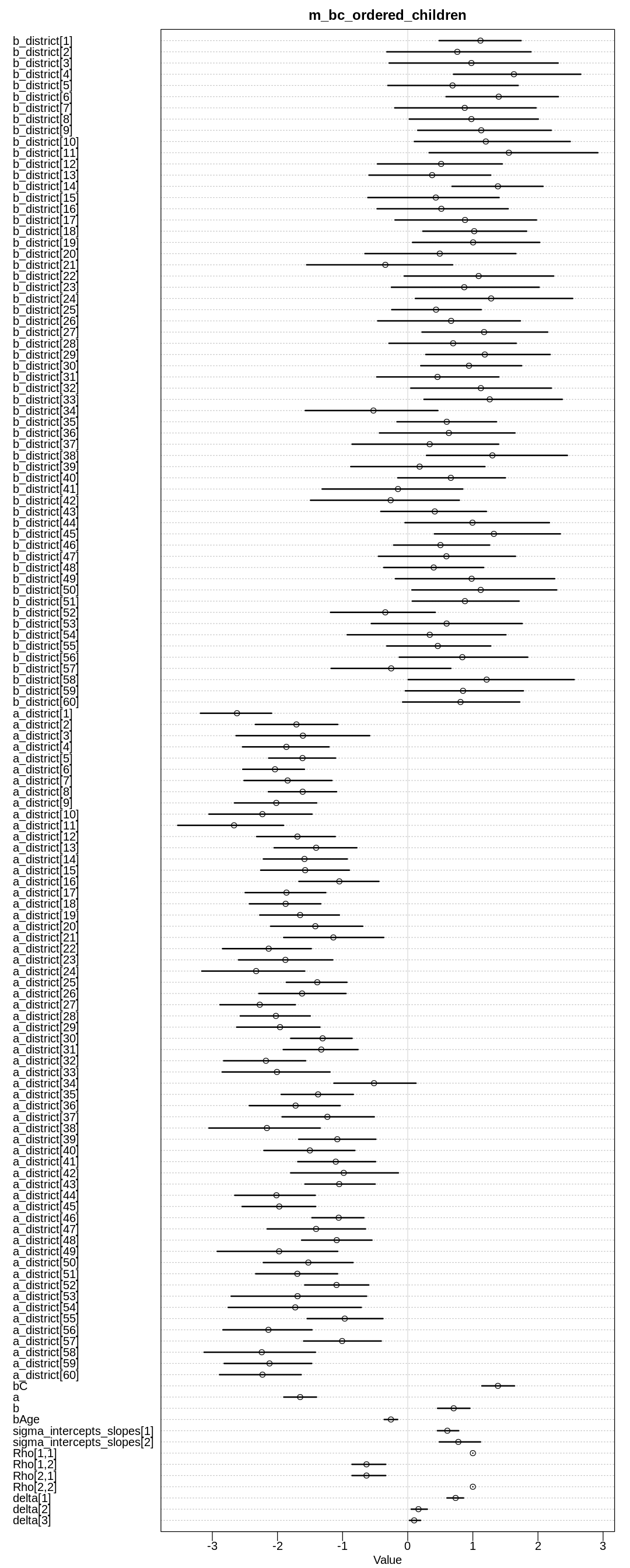
Notice in the summary of this data frame, above, that the women surveyed had a minimum of one and
a maximum of four children. It appears the maximum jump in likelihood of a woman using contraception
occurs after having the second child.
14H4. Varying effects models are useful for modeling time series, as well as spatial clustering.
In a time series, the observations cluster by entities that have continuity through time, such as
individuals. Since observations within individuals are likely highly correlated, the multilevel
structure can help quite a lot. You’ll use the data in data(Oxboys), which is 234 height
measurements on 26 boys from an Oxford Boys Club (I think these were like youth athletic leagues?),
at 9 different ages (centered and standardized) per boy. You’ll be interested in predicting
height, using age, clustered by Subject (individual boy). Fit a model with varying intercepts
and slopes (on age), clustered by Subject. Present and interpret the parameter estimates. Which
varying effect contributes more variation to the heights, the intercept or the slope?
data(Oxboys)
ox <- Oxboys
Answer. A head and summary of the Oxboys data.frame (no help exists):
display(head(ox))
display(summary(ox))
| Subject | age | height | Occasion | |
|---|---|---|---|---|
| <int> | <dbl> | <dbl> | <int> | |
| 1 | 1 | -1.0000 | 140.5 | 1 |
| 2 | 1 | -0.7479 | 143.4 | 2 |
| 3 | 1 | -0.4630 | 144.8 | 3 |
| 4 | 1 | -0.1643 | 147.1 | 4 |
| 5 | 1 | -0.0027 | 147.7 | 5 |
| 6 | 1 | 0.2466 | 150.2 | 6 |
    Subject          age               height         Occasion
 Min.   : 1.0   Min.   :-1.00000   Min.   :126.2   Min.   :1
 1st Qu.: 7.0   1st Qu.:-0.46300   1st Qu.:143.8   1st Qu.:3
 Median :13.5   Median :-0.00270   Median :149.5   Median :5
 Mean   :13.5   Mean   : 0.02263   Mean   :149.5   Mean   :5
 3rd Qu.:20.0   3rd Qu.: 0.55620   3rd Qu.:155.5   3rd Qu.:7
 Max.   :26.0   Max.   : 1.00550   Max.   :174.8   Max.   :9
Fitting the model:
ox_dat <- list(
  Subject = ox$Subject,
  Age = ox$age,
  Height = ox$height
)
m_ox <- ulam(
  alist(
    Height ~ dnorm(mu, sigma),
    mu <- a_boy[Subject] + b_boy[Subject] * Age,
    c(a_boy, b_boy)[Subject] ~ multi_normal(c(a, b), Rho, sigma_intercepts_slopes),
    a ~ normal(0, 1),
    b ~ normal(0, 0.5),
    sigma_intercepts_slopes ~ exponential(1),
    Rho ~ lkj_corr(2),
    sigma ~ normal(0, 2)
  ),
  data = ox_dat, chains = 4, cores = 4, log_lik = TRUE
)
display(precis(m_ox, depth=3), mimetypes="text/plain")
iplot(function() {
  plot(precis(m_ox, depth=3), main="m_ox")
}, ar=0.7)
                           mean        sd         5.5%        94.5%
b_boy[1]                     7.137421  0.3470028    6.593290    7.685841
b_boy[2]                     5.481388  0.3354717    4.953505    6.018759
b_boy[3]                     4.871198  0.3242252    4.349729    5.384686
b_boy[4]                     9.248308  0.3286225    8.723941    9.775897
b_boy[5]                     6.262325  0.3430345    5.720164    6.794605
b_boy[6]                     4.065094  0.3414588    3.507843    4.625468
b_boy[7]                     5.057129  0.3254772    4.550538    5.600158
b_boy[8]                     6.472143  0.3409617    5.918703    7.011299
b_boy[9]                     6.008275  0.3482750    5.451821    6.546127
b_boy[10]                    3.822563  0.3308904    3.288179    4.352849
b_boy[11]                    8.414984  0.3420993    7.896069    8.966929
b_boy[12]                    7.003539  0.3169374    6.496528    7.504444
b_boy[13]                    8.411397  0.3244596    7.903736    8.921488
b_boy[14]                    8.584270  0.3479208    8.024445    9.140723
b_boy[15]                    7.084154  0.3311591    6.576340    7.612390
b_boy[16]                    4.632670  0.3351358    4.111953    5.170819
b_boy[17]                    8.503973  0.3483309    7.942851    9.053097
b_boy[18]                    5.993513  0.3326001    5.483076    6.526629
b_boy[19]                    8.976750  0.3399502    8.432994    9.514783
b_boy[20]                    4.472405  0.3421088    3.928483    5.025561
b_boy[21]                    7.459345  0.3350197    6.935254    7.996470
b_boy[22]                    8.026042  0.3425854    7.475904    8.563561
b_boy[23]                    7.155082  0.3293630    6.633925    7.688765
b_boy[24]                    6.758130  0.3489079    6.217386    7.324170
b_boy[25]                    4.119345  0.3261452    3.618808    4.628240
b_boy[26]                    5.611484  0.3198873    5.097121    6.124518
a_boy[1]                   148.113666  0.2214899  147.760040  148.470348
a_boy[2]                   142.852459  0.2277650  142.483513  143.220769
a_boy[3]                   155.647841  0.2273460  155.290838  156.013241
a_boy[4]                   165.077054  0.2245467  164.719447  165.438460
⋮                          ⋮           ⋮          ⋮           ⋮
a_boy[6]                   146.7816740 0.21651718 146.4285482 147.1306175
a_boy[7]                   146.1256625 0.22946990 145.7590553 146.4807607
a_boy[8]                   148.2952714 0.22680539 147.9407225 148.6682984
a_boy[9]                   138.1430095 0.21399152 137.8103545 138.4762010
a_boy[10]                  130.2641576 0.22281089 129.9045046 130.6156562
a_boy[11]                  150.0505071 0.22596823 149.6941118 150.4049100
a_boy[12]                  156.8038612 0.21954019 156.4661561 157.1615807
a_boy[13]                  156.0790796 0.22703441 155.7234655 156.4528918
a_boy[14]                  159.4761872 0.22282774 159.1283867 159.8305711
a_boy[15]                  144.2824583 0.22543143 143.9169227 144.6406060
a_boy[16]                  147.5473591 0.22410248 147.1885303 147.8914143
a_boy[17]                  142.9797313 0.22542690 142.6231427 143.3483465
a_boy[18]                  151.1778984 0.21780214 150.8322288 151.5216472
a_boy[19]                  164.5871053 0.23456883 164.2127483 164.9628855
a_boy[20]                  151.4691104 0.21856394 151.1150465 151.8145878
a_boy[21]                  150.5169563 0.21928624 150.1524631 150.8591893
a_boy[22]                  154.5666657 0.22340787 154.2099223 154.9231753
a_boy[23]                  151.0604161 0.23528629 150.6893835 151.4446547
a_boy[24]                  153.1466540 0.23028317 152.7808444 153.4993456
a_boy[25]                  139.2048731 0.21329264 138.8642392 139.5451884
a_boy[26]                  137.9953264 0.21980365 137.6500644 138.3334579
a                            0.6537408 1.01336819  -0.9283681   2.2715824
b                            0.1333895 0.48955902  -0.6369618   0.9309867
sigma_intercepts_slopes[1]  74.6934922 4.68032793  67.4601565  82.1614231
sigma_intercepts_slopes[2]   3.5748334 0.32779123   3.0554130   4.1134228
Rho[1,1]                     1.0000000 0.00000000   1.0000000   1.0000000
Rho[1,2]                     0.8880278 0.03607893   0.8246749   0.9352457
Rho[2,1]                     0.8880278 0.03607893   0.8246749   0.9352457
Rho[2,2]                     1.0000000 0.00000000   1.0000000   1.0000000
sigma                        0.6647896 0.03639783   0.6084315   0.7252927
                           n_eff    Rhat4
b_boy[1]                   3528.749 0.9999860
b_boy[2]                   4168.444 0.9996024
b_boy[3]                   2986.183 0.9986559
b_boy[4]                   3184.555 0.9988569
b_boy[5]                   4628.295 0.9986748
b_boy[6]                   3157.599 0.9986585
b_boy[7]                   3067.210 1.0018310
b_boy[8]                   3605.736 0.9991257
b_boy[9]                   3235.929 0.9989471
b_boy[10]                  3524.432 0.9991593
b_boy[11]                  3555.813 0.9985748
b_boy[12]                  3295.006 0.9983287
b_boy[13]                  3261.745 0.9985648
b_boy[14]                  3638.736 1.0001942
b_boy[15]                  3922.221 0.9984418
b_boy[16]                  3387.989 0.9991188
b_boy[17]                  3695.833 0.9999522
b_boy[18]                  4232.337 0.9991695
b_boy[19]                  3671.879 0.9997550
b_boy[20]                  2721.981 0.9992497
b_boy[21]                  3176.938 0.9983887
b_boy[22]                  3561.369 0.9994862
b_boy[23]                  3902.230 0.9987558
b_boy[24]                  3227.228 1.0002230
b_boy[25]                  3818.300 0.9996149
b_boy[26]                  3410.292 1.0004828
a_boy[1]                   4561.809 0.9987926
a_boy[2]                   3535.504 0.9998455
a_boy[3]                   3005.947 0.9996865
a_boy[4]                   3959.527 0.9986625
⋮                          ⋮        ⋮
a_boy[6]                   3586.519 0.9993449
a_boy[7]                   3621.095 0.9999323
a_boy[8]                   2529.734 0.9983566
a_boy[9]                   2600.322 0.9996230
a_boy[10]                  3124.062 0.9989691
a_boy[11]                  3161.117 0.9988722
a_boy[12]                  3231.492 0.9985778
a_boy[13]                  3953.531 0.9989110
a_boy[14]                  2868.897 0.9992057
a_boy[15]                  3993.774 1.0000635
a_boy[16]                  3126.013 0.9988499
a_boy[17]                  3317.890 0.9990095
a_boy[18]                  3539.491 0.9989600
a_boy[19]                  2805.662 0.9986506
a_boy[20]                  3454.852 0.9985530
a_boy[21]                  3114.616 0.9984869
a_boy[22]                  3719.990 1.0003180
a_boy[23]                  3721.650 0.9988570
a_boy[24]                  3812.427 0.9991344
a_boy[25]                  3265.778 0.9990980
a_boy[26]                  3590.703 0.9994189
a                          4519.370 0.9981847
b                          2040.379 0.9995646
sigma_intercepts_slopes[1] 2474.403 0.9992004
sigma_intercepts_slopes[2] 2001.709 0.9986325
Rho[1,1]                        NaN       NaN
Rho[1,2]                   2216.757 0.9990147
Rho[2,1]                   2216.757 0.9990147
Rho[2,2]                        NaN       NaN
sigma                      2050.545 1.0026862
The intercepts term contributes much more to the heights than the slopes. Notice the b_boy terms
are the maximum that the slopes can contribute to mu since Age is at most equal one.
14H5. Now consider the correlation between the varying intercepts and slopes. Can you explain its value? How would this estimated correlation influence your predictions about a new sample of boys?
Answer. The correlation is positive, because more positive intercepts are associated with more positive slopes. That is, boys who are on average taller also grow faster.
14H6. Use mvrnorm (in library(MASS)) or rmvnorm (in library(mvtnorm)) to simulate a new
sample of boys, based upon the posterior mean values of the parameters. That is, try to simulate
varying intercepts and slopes, using the relevant parameter estimates, and then plot the predicted
trends of height on age, one trend for each simulated boy you produce. A sample of 10 simulated boys
is plenty, to illustrate the lesson. You can ignore uncertainty in the posterior, just to make the
problem a little easier. But if you want to include the uncertainty about the parameters, go for it.
Note that you can construct an arbitrary variance-covariance matrix to pass to either mvrnorm or
rmvnorm with something like:
R code 14.54
S <- matrix( c( sa^2 , sa*sb*rho , sa*sb*rho , sb^2 ) , nrow=2 )
where sa is the standard deviation of the first variable, sb is the standard deviation of the
second variable, and rho is the correlation between them.
Answer. The expected plot:
post <- extract.samples(m_ox)
Mu_est <- c(mean(post$a), mean(post$b))
rho_est <- mean(post$Rho[,1,2])
sa_est <- mean(post$sigma_intercepts_slopes[,1])
sb_est <- mean(post$sigma_intercepts_slopes[,2])
cov_ab <- sa_est*sb_est*rho_est
Sigma_est <- matrix(c(sa_est^2, cov_ab, cov_ab, sb_est^2), nrow=2)

library(MASS)
set.seed(5)
N_boys <- 10
vary_effects <- mvrnorm(N_boys, Mu_est, Sigma_est)

iplot(function() {
  plot(NULL, main="Posterior predictive plot, 10 simulated boys",
    xlab="age", ylab="height",
    xlim=c(-1.1, 1.1),
    ylim=c(min(vary_effects[,1] - vary_effects[,2]) - 10, max(vary_effects[,1] + vary_effects[,2]) + 10)
  )
  for (idx in 1:N_boys)
    abline(a=vary_effects[idx, 1], b=vary_effects[idx, 2])
})
The lesson here is that vague priors can kill predictive power, and that in situations like this one
the priors have a strong influence on the results. In the previous plot the priors on a and b
were copied and pasted from another model:
These are clearly unreasonable. If we fix these priors we get a much better result:
m_ox2 <- ulam(
  alist(
    Height ~ dnorm(mu, sigma),
    mu <- a_boy[Subject] + b_boy[Subject] * Age,
    c(a_boy, b_boy)[Subject] ~ multi_normal(c(a, b), Rho, sigma_intercepts_slopes),
    a ~ normal(150, 40),
    b ~ normal(40, 40),
    sigma_intercepts_slopes ~ exponential(1),
    Rho ~ lkj_corr(2),
    sigma ~ normal(0, 2)
  ),
  data = ox_dat, chains = 4, cores = 4, log_lik = TRUE
)
display(precis(m_ox2, depth=3), mimetypes="text/plain")
iplot(function() {
  plot(precis(m_ox2, depth=3), main="m_ox2")
}, ar=0.7)

post <- extract.samples(m_ox2)
Mu_est <- c(mean(post$a), mean(post$b))
rho_est <- mean(post$Rho[,1,2])
sa_est <- mean(post$sigma_intercepts_slopes[,1])
sb_est <- mean(post$sigma_intercepts_slopes[,2])
cov_ab <- sa_est*sb_est*rho_est
Sigma_est <- matrix(c(sa_est^2, cov_ab, cov_ab, sb_est^2), nrow=2)

library(MASS)
set.seed(5)
N_boys <- 10
vary_effects <- mvrnorm(N_boys, Mu_est, Sigma_est)

iplot(function() {
  plot(NULL, main="Posterior predictive plot, 10 simulated boys",
    xlab="age", ylab="height",
    xlim=c(-1.1, 1.1),
    ylim=c(min(vary_effects[,1] - vary_effects[,2]) - 10, max(vary_effects[,1] + vary_effects[,2]) + 10)
  )
  for (idx in 1:N_boys)
    abline(a=vary_effects[idx, 1], b=vary_effects[idx, 2])
})
                           mean        sd           5.5%        94.5%
b_boy[1]                     7.122827  0.3322087      6.583848    7.655954
b_boy[2]                     5.460675  0.3309538      4.937802    6.000382
b_boy[3]                     4.934086  0.3372113      4.401751    5.461362
b_boy[4]                     9.290755  0.3408733      8.753078    9.830426
b_boy[5]                     6.279010  0.3414299      5.738504    6.831309
b_boy[6]                     4.107758  0.3332389      3.586919    4.640147
b_boy[7]                     5.064438  0.3433725      4.520589    5.604039
b_boy[8]                     6.463974  0.3402083      5.927326    6.991294
b_boy[9]                     5.958746  0.3234855      5.461362    6.483401
b_boy[10]                    3.754424  0.3422636      3.209548    4.298276
b_boy[11]                    8.376141  0.3459315      7.827744    8.901756
b_boy[12]                    7.037235  0.3251566      6.529788    7.552236
b_boy[13]                    8.421781  0.3320623      7.887876    8.969216
b_boy[14]                    8.606473  0.3324009      8.088091    9.125618
b_boy[15]                    7.052871  0.3329311      6.496938    7.582998
b_boy[16]                    4.648309  0.3358858      4.131960    5.187072
b_boy[17]                    8.427887  0.3242495      7.909494    8.945488
b_boy[18]                    6.003476  0.3500593      5.438516    6.563315
b_boy[19]                    9.016830  0.3303680      8.477545    9.540540
b_boy[20]                    4.527208  0.3365359      3.984102    5.066829
b_boy[21]                    7.447827  0.3292831      6.908307    7.986375
b_boy[22]                    8.023659  0.3309146      7.499065    8.543218
b_boy[23]                    7.152485  0.3387705      6.633455    7.682342
b_boy[24]                    6.784337  0.3493435      6.229581    7.355831
b_boy[25]                    4.106523  0.3317459      3.575951    4.634723
b_boy[26]                    5.557906  0.3539407      4.985938    6.127773
a_boy[1]                   148.125102  0.2240055    147.756752  148.485698
a_boy[2]                   142.868576  0.2203292    142.518234  143.210920
a_boy[3]                   155.632299  0.2254481    155.266723  155.978131
a_boy[4]                   165.064997  0.2285159    164.709111  165.443212
⋮                          ⋮           ⋮            ⋮           ⋮
a_boy[6]                   146.7861098 2.194073e-01 146.4384452 147.1318658
a_boy[7]                   146.1210404 2.337751e-01 145.7343224 146.4824160
a_boy[8]                   148.2930374 2.243746e-01 147.9392885 148.6591341
a_boy[9]                   138.1513979 2.313018e-01 137.7888748 138.5179245
a_boy[10]                  130.2768959 2.161344e-01 129.9233319 130.6063412
a_boy[11]                  150.0537839 2.192917e-01 149.7113235 150.4125345
a_boy[12]                  156.7994271 2.247133e-01 156.4529092 157.1583169
a_boy[13]                  156.0717378 2.231343e-01 155.6971782 156.4154992
a_boy[14]                  159.4622504 2.268403e-01 159.1051252 159.8277467
a_boy[15]                  144.2840014 2.288367e-01 143.9157850 144.6475227
a_boy[16]                  147.5418819 2.208381e-01 147.1855594 147.8994849
a_boy[17]                  142.9979601 2.268262e-01 142.6356783 143.3596771
a_boy[18]                  151.1794610 2.169724e-01 150.8242030 151.5177369
a_boy[19]                  164.5677562 2.193259e-01 164.2165483 164.9211439
a_boy[20]                  151.4573911 2.289793e-01 151.1095460 151.8243764
a_boy[21]                  150.5201332 2.205926e-01 150.1666056 150.8674592
a_boy[22]                  154.5665399 2.197841e-01 154.2112713 154.9120035
a_boy[23]                  151.0684985 2.245058e-01 150.7159832 151.4270030
a_boy[24]                  153.1327253 2.242584e-01 152.7759679 153.4905381
a_boy[25]                  139.2209405 2.212194e-01 138.8686246 139.5646712
a_boy[26]                  138.0036029 2.302090e-01 137.6423519 138.3753935
a                          149.3923945 1.455555e+00 147.0672831 151.7613879
b                            6.5311084 3.284126e-01   6.0277505   7.0514299
sigma_intercepts_slopes[1]   7.3280618 8.909815e-01   6.0736747   8.8576264
sigma_intercepts_slopes[2]   1.6304761 2.332820e-01   1.2976833   2.0271578
Rho[1,1]                     1.0000000 0.000000e+00   1.0000000   1.0000000
Rho[1,2]                     0.5257282 1.299665e-01   0.2859021   0.7119550
Rho[2,1]                     0.5257282 1.299665e-01   0.2859021   0.7119550
Rho[2,2]                     1.0000000 7.984801e-17   1.0000000   1.0000000
sigma                        0.6652505 3.387909e-02   0.6144083   0.7236621
                           n_eff    Rhat4
b_boy[1]                   3397.241 0.9993882
b_boy[2]                   3824.896 0.9991548
b_boy[3]                   4551.947 0.9986551
b_boy[4]                   4846.730 0.9984812
b_boy[5]                   3796.926 0.9981290
b_boy[6]                   3969.628 0.9994277
b_boy[7]                   3717.169 0.9995144
b_boy[8]                   3885.725 0.9988696
b_boy[9]                   3130.566 0.9982011
b_boy[10]                  3829.525 0.9996160
b_boy[11]                  4275.056 0.9990806
b_boy[12]                  3486.493 0.9986922
b_boy[13]                  3565.861 0.9988748
b_boy[14]                  5191.336 0.9989458
b_boy[15]                  3540.452 0.9982362
b_boy[16]                  3274.932 0.9995209
b_boy[17]                  3718.099 0.9982985
b_boy[18]                  3729.188 0.9992369
b_boy[19]                  4254.105 0.9986004
b_boy[20]                  3826.369 0.9985832
b_boy[21]                  3864.268 0.9989389
b_boy[22]                  3111.481 0.9993075
b_boy[23]                  3595.851 0.9989247
b_boy[24]                  3738.130 0.9983798
b_boy[25]                  3236.979 0.9988405
b_boy[26]                  4879.405 0.9984281
a_boy[1]                   3237.550 0.9987787
a_boy[2]                   4049.226 0.9986528
a_boy[3]                   3117.776 0.9985072
a_boy[4]                   5100.197 0.9987063
⋮                          ⋮        ⋮
a_boy[6]                   3308.713 1.0001489
a_boy[7]                   3880.149 0.9990667
a_boy[8]                   3317.791 0.9991302
a_boy[9]                   5297.428 0.9994021
a_boy[10]                  4105.215 1.0000839
a_boy[11]                  3896.860 0.9988511
a_boy[12]                  3777.433 0.9989543
a_boy[13]                  4259.095 0.9990450
a_boy[14]                  4502.372 0.9996217
a_boy[15]                  4221.052 0.9987526
a_boy[16]                  4264.674 0.9988805
a_boy[17]                  3706.006 0.9986395
a_boy[18]                  3493.254 0.9986243
a_boy[19]                  3833.874 0.9992270
a_boy[20]                  3961.773 0.9986611
a_boy[21]                  4278.342 0.9984816
a_boy[22]                  4313.655 0.9987957
a_boy[23]                  5199.071 0.9988071
a_boy[24]                  4171.203 0.9989638
a_boy[25]                  4217.568 0.9995400
a_boy[26]                  4517.137 0.9988017
a                          2719.812 0.9993785
b                          2536.216 1.0007571
sigma_intercepts_slopes[1] 2971.258 0.9986441
sigma_intercepts_slopes[2] 2646.944 0.9995006
Rho[1,1]                        NaN       NaN
Rho[1,2]                   2607.412 0.9985915
Rho[2,1]                   2607.412 0.9985915
Rho[2,2]                   1956.060 0.9979980
sigma                      2380.168 0.9985868