Review: 2nd Edition

Summary

There are a lot of typos and errors in the second edition. Take the attitude of ignoring these early on or finding a way to only mark them for your own sake. In the more detailed review below, you will see obvious errors marked with ERROR. This list is largely incomplete; it misses many minor errors (i.e. typos) later in the book as they become too tiresome to collect. If you don’t believe me, see all the unresolved open issues in the author’s GitHub repository.

The ERRATA is empty because (of course) GitHub issues are not being addressed. The absolute number of errors is probably also part of the problem. This is a shame because even an incomplete errata makes reading a book easier; you should often keep an errata open when you read a textbook to avoid puzzling over an issue someone else has already identified and explained. If a book doesn’t have an errata, either the author never makes mistakes or they don’t have the time.

VitalSource

The ebook format (VitalSource) is quite limited. The VitalSource pages are painfully slow to load; I would load several chapters in different tabs at once (in Firefox, use Alt-D then Alt-Enter to duplicate a tab). You’ll need a tab for global search in the book as well.

The VitalSource format doesn’t display page numbers well and can only be navigated with a mouse (unlike an HTML page). Some errors only appear in the VitalSource and not in the pbook (printed book). If you’re reading the VitalSource (as you must if you want to use a digital copy) then you’re also going to need to get used to its rendering of equations, which is horrendous (see e.g. section 4.4.1 or 12.3.2).

In my experience, it was best to ‘Reset to Publisher Format’ and use my browser to change the text size.

Other publishers (like MAA) provide you with a PDF that is clearly marked with your name to prevent distribution. You can find one bootlegged pdf version of Statistical Rethinking Ed. 2 (SR2) online (from Dec. 2019), missing significant content and with even more errors. The author has apparently offered online courses in the past to get a pdf.

All external links are broken in the VitalSource version of this book. That is, you must copy and paste links rather than click on them. That is, the blue links internal to the book are functional, but blue links to external websites are broken.

Strengths

The book is entertaining, which can make it easier to remember concepts. As advertised, it’s driven by many Worked examples. In general, it also focuses on the forest rather than the trees. These are the primary ways it tries to distinguish itself from more standard textbooks on Bayesian analysis such as BDA3. The author seems to be heavily influenced by Gelman, based on both his references and how the book relies on Stan (developed by Gelman).

The chapter layouts, with Rcode text boxes interspersed, is similar to a Jupyter notebook but without being directly executable. Unfortunately not being executable means the chapter code doesn’t actually run without a number of fixes. The advantage to this approach is users can work in a plain text editor rather than a browser, but this doesn’t in itself imply the code shouldn’t be runnable.

Personal Workflow

Start by getting models working with MCMC (ulam), which provides a lot more debugging information and is capable of estimating non-Gaussian posteriors. Once you’re happy with the results, check that quap provides the same answer and switch to it so scripts run faster.

Prefer to source R files from the shell rather than running the publish script when you’re debugging issues. Many errors/warnings are swallowed otherwise.

See also davidvandebunte/rethinking: GitHub.

2.3. Components of the model

2.3.2. Definitions

By far the most confusing definition given here is for the likelihood. In this book, a ‘likelihood’ will refer to a distribution function assigned to an observed variable. In this section, for example, the ‘likelihood’ is the binomial distribution. According to the author, this is the language used in ‘conventional’ statistics as well. The author often calls this the ‘likelihood’ but it is a function, of course, because any probability distribution is a function.

In non-Bayesian statistics and in particular on Wikipedia the definition of the likelihood function is completely different and denoted with \(\mathcal{L}\). See the author’s footnote and Likelihood function.

3.3. Sampling to simulate prediction

3.3.1. Dummy data

In this way, Bayesian models are always generative, capable of simulating predictions.

Bayesian models are always generative, capable of simulating observations.

If you search for generative you’ll see the author “defines” it again at the start of section 3.3.2 (correctly this time). See also Define generative model.

4.3. Gaussian model of height

4.3.1. The data

We can also use rethinking’s precis summary function, which we’ll use to summarize posterior distributions later on:

This function is not introduced or documented well; it will be taught by example. The name refers to precision as in Accuracy and precision.

4.4.3. Interpreting the posterior distribution

ERROR:

What link will do is take your quap approximation, sample from the posterior distribution, and then compute \(\mu\) for each case in the data and sample from the posterior distribution.

link doesn’t sample from the posterior distribution twice. This sentence should read:

What link will do is take your quap approximation, sample from the posterior distribution, and then compute \(\mu\) for each case in the data.

The function sim is equivalent to inference (see Statistical inference) in machine learning, but on the training data.

4.4.3.5. Prediction intervals.

ERROR:

This part of R code 4.61 is wrong:

# draw HDPI region for line
shade( mu.HPDI , weight.seq )

It should be (see Issue #319):

# draw PI region for line
shade( mu.PI , weight.seq )

4.5. Curves from lines

4.5.1. Polynomial regression.

It is standard practice to STANDARDIZE variables but the explanation given here isn’t particularly helpful. Consider scale provided by the R language. When should you set center to TRUE? When should you set scale to TRUE? The author’s function standardize will show up without explanation later in the book, but all it adds to scale (if you look at it) is a little type coercion.

See also Feature scaling. This article uses the terms ‘normalization’ and ‘standardization’ in a way that almost match the author’s normalize and standardize functions.

See also:

• Normalization (statistics).

• Understanding scale in R - SO.

Perhaps one way to look at this is as providing priors to the machine about what is big and small, though in theory it could figure it out from the data. In other cases, the model may make assumptions about predictors being on the same scale. Is there a way to communicate bounds such as that the numbers are percentages in question 11H4?

You often run into failures to fit because variables are not standardized. For example, quap asks for a starting point or ulam spits many warnings. In most of these cases, you aren’t supplying reasonable priors. It may be standardization is an easy way to get parameters on the same scale and indirectly provide these priors in a simple way, without the work of doing a prior predictive simulation. That is, could standardization be a way to avoid the work of supplying reasonable priors?

The other advantage of standardization is you can look at precis output and compare parameter values because all your parameters are about on the same scale. Are you preferring the convenience of using a single parameter scale on this plot too much? You may also be avoiding posterior predictive simulation, preferring to look at parameter values instead only because it’s easier to look at parameter values than work on the outcome scale.

See also this comment in section 14.3:

We standardized the variables, so we can use our default priors for standardized linear regression.

5.1. Spurious assocation

ERROR:

we can use extract.prior and link as in the previous chapter.

(extract.prior has only been mentioned in the preface)

5.1.3. Multiple regression notation

ERROR:

R for marriage rate and A for age at marriage

(actually using M for marriage rate)

5.1.4. Approximating the posterior

ERROR:

with plenty of probability of [sic] both sides of zero.

5.2. Masked relationship

ERROR:

we can do better by both [sic] tightening the α prior so that it sticks closer to zero.

5.3.1. Binary categories

ERROR:

Vector (and matrix) parameters are hidden by precies [sic] by default, because

6.3. Collider bias

6.3.1. Collider of false sorrow.

ERROR: See:

This is just the categorical variable strategy from Chapter 4.

The categorical variable strategy is discussed in Section 5.3.

This section is naturally hard to understand, so here’s an extra explanation for why conditioning on marriage leads to a negative association between age and happiness. First, lets assume we know you’re married. If you’re young, then it’s quite likely you’re happier than average because you got married so young. If you’re old, then it may only be time that led to you getting married. So in summary, being older is a good indication you’re unhappy (a negative association). Second, lets assume we know you’re unmarried. If you’re young, then you may simply not have had enough time to get married. If you’re old and still unmarried, it’s more likely you are an unhappy person and so the time treatment didn’t lead you to getting married. So in summary, being older is a good indication you’re unhappy (a negative association).

Said yet another way, consider Figure 6.4. From age 20 to 30, the average of the blue bubbles is about 1. At age 60, the average of the blue bubbles is closer to zero. Now consider the white bubbles. From 20 to 30, the average of the white bubbles is close to zero. At age 60, the average is closer to -1.

7.2. Entropy and accuracy

7.2.3. From entropy to accuracy.

If we’re going from Earth to Mars, we’re an Earthling with certain priors (vice versa, a Martian).

From this perspective, by using a high entropy distribution to approximate an unknown true distribution, we’re less surprised by any particular observation because in general we don’t expect anything unlikely. The Earthling was from the higher entropy planet, and so wasn’t as surprised by travel.

When we use a higher entropy distribution we’re potentially reducing the cross entropy by reducing the \(log(q_i)\) terms (in particular, the sum of the terms will definitely be reduced). We’re not guaranteed to reduce the cross entropy (and therefore the KL divergence) though, because by increasing the entropy of \(q\) we may be making it dissimilar to \(p\) in a way that increases a term where \(p_i\) is large. Read question 7H3 for a numerical example.

7.2.4. Estimating divergence.

Mnemonics: Notice that p is the real thing, the ‘true’ model. The p stands for probability; the p is the symbol we normally use. The q (and r) models are an the approximation, the model we are evaluating (the next letters in the alphabet). We use \(D\) (in e.g. \(D_{train}\)) for both divergence and deviance.

ERROR: See this quote:

In that case, most of p just subtracts out, because there is a \(E[log(p_i)]\) term in the divergence of both q and r.

The term of ‘most of’ should be removed, this is clearly a complete cancellation:

\[\begin{split} \begin{align} D_{KL}(p,q) & = H(p,q) - H(p) \\ D_{KL}(p,r) & = H(p,r) - H(p) \\ D_{KL}(p,q) - D(p,r) & = H(p,q) - H(p,r) \\ \end{align} \end{split}\]

A log-probability score (or the lppd) estimates the cross entropy.

These concepts on a number line:

7.2.5. Scoring the right data

The true model has three parameters: \( \mu_{i}, \beta_1, \beta_2 \)

ERROR: The ‘Overthinking’ box refers to sim.train.test, which is from the first version of the book.

7.3. Golem taming: regularization

The term ‘regularization’ in this context doesn’t refer to the kind of regularization common in other areas of machine learning and deep learning, where regularization is a restriction on the values that weights can take on, enforced by an addition to the loss term.

See Regularization (mathematics).

7.4. Predicting predictive accuracy

7.4.1. Cross-validation

Importance sampling with PSIS is connected to anomaly detection in deep learning; they both provide outlier warnings.

7.4.2. Information criteria

ERROR:

dominate AIC is [sic] every context

7.4.3. Comparing CV, PSIS, and WAIC

ERROR:

The bottom row shows 1000 simulations with N = 1000 [sic, should be N = 100].

8.2. Symmetry of interactions

To relate these equations to the form of the equations in section 8.3, where equations have four terms:

\[\begin{split} \begin{align} \mu_i & = (2 - CID_i)(\alpha_1 + \beta_1\left(r_i - \bar{r}\right)) + \ (CID_i - 1)(\alpha_2 + \beta_2\left(r_i - \bar{r}\right)) \\ \mu_i & = (2\alpha_1 - \alpha_2) + (\alpha_2 - \alpha_1)CID_i + \ (2\beta_1 - \beta_2)\left(r_i - \bar{r}\right) + \ (\beta_2 - \beta_1)CID_{i}\left(r_i - \bar{r}\right) \end{align} \end{split}\]

See also answer 8E3 (scenario 2).

ERROR:

(unless we are exactly at the average ruggedness \(\bar{r}\))

If we are exactly at the average ruggedness, we still need to know we are at the average ruggedness to predict how switching a nation to Africa will affect prediction.

8.3. Continuous interactions

ERROR:

When we have two variable, [sic]

9.3. Hamiltonian Monte Carlo

ERROR: The definition of U_gradient uses different symbols (a, b, k, d) leading to Gaussian distributions with a standard deviation of 1.0 rather than 0.5.

10.1. Maximum entropy

For a list of maximum entropy distributions see Maximum entropy probability distribution.

10.2. Generalized linear models

For a list of common link functions see Link function.

10.2.3. Omitted variable bias again

An example would seriously help this explanation. You’ll see an example of exactly this situation in section 15.2.1. (perhaps what the author is thinking of as he writes this).

11.1. Binomial regression

We’ll work some examples using quap

For commentary on times you should not use quap see:

• The Overthinking box in section 4.3.4

• The Rethinking box in section 2.4.4

The typical network in deep learning will be based on MLE (i.e. quap). If you want to add another predictor to this kind of network you need to ask whether you expect the posterior to be Gaussian or you may struggle to get optimization (i.e. inference) to work. You also need to confirm your priors are symmetric (see 11M7) again so that optimization works. Because MCMC is much more time expensive than MLE, you may not have a choice.

If you have the time, you can compare a quap and ulam fit to confirm quap is good enough. If there is no difference in inference, then clearly it doesn’t matter. Another major advantage of ulam over quap is it will report errors when you’re struggling to fit.

11.1.1 Logistic regression: Prosocial chimpanzees

If you’re not familiar with xtab, duck !w crosstab.

11.1.2. Relative shark and absolute deer.

The author refers to what is more commonly known as the Odds ratio as ‘Proportional Odds’ in this section.

The example in the Overthinking box isn’t particularly clear. If the odds \(p/(1-p)\) are 1/100 then doubling them should produce odds of 2/100, not 2/99. This moves p from approximately:

\[ (1/100)/(1 + 1/100) \approx 0.0099 \]

to:

\[ (2/100)/(1 + 2/100) \approx 0.0196 \]

11.1.3. Aggregated binomial: Chimpanzees again, condensed.

ERROR:

Here are the results for the first two chimpanzees:

These are definitely not the results for the first two chimpanzees; they’re the results for the first treatment.

11.1.4. Aggregated binomial: Graduate school admissions

ERROR:

The function coerce_index can do this for us, using the dept factor as input.

The R code box never uses this function.

11.2. Poisson regression

11.2.1. Example: Oceanic tool complexity.

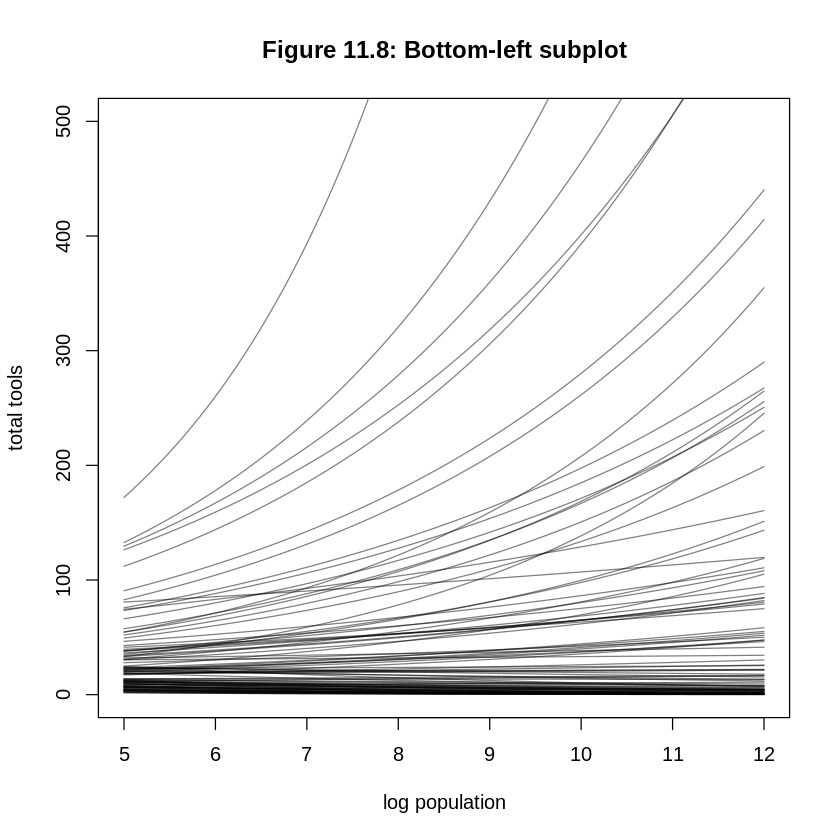
ERROR: The subplot titles in Figure 11.8 are confused. In the bottom two subplots, the titles should be a ~ dnorm(3, 0.5), b ~ dnorm(0, 0.2) rather than b ~ dnorm(3, 0.5), b ~ dnorm(0, 0.2). It’s not clear why a is not specified in the top two subplots; the plots are reproducible with a ~ dnorm(3, 0.5).

The more significant mistake in this section is in how it attempts to compare the standardized log population and log population scales. The top right and bottom left subplots of Figure 11.8 should be the same with a differently labeled x-axis if all we’re doing is scaling. What the bottom-left of Figure 11.8 actually produces is a different view of the prior on the standardized log population scale. To understand this, consider this code to reproduce the bottom-left subplot. This code only changes xlim and ylim in R code 11.42 rather than switching to the more complicated approach in R code 11.43:

library(IRdisplay)
suppressPackageStartupMessages(library(rethinking))

## R code 11.42
set.seed(10)
N <- 100
a <- rnorm(N, 3, 0.5)
b <- rnorm(N, 0, 0.2)
plot(NULL, xlim = c(5, 12), ylim = c(0, 500), main='Figure 11.8: Bottom-left subplot',
   xlab='log population', ylab='total tools')
for (i in 1:N) curve(exp(a[i] + b[i] * x), add = TRUE, col = grau())

The a and b priors are being selected for a standardized log population scale. You can’t use them with a log population scale, or you would have to change them. One of the reasons we like to standardize variables is so that it’s easier to select priors; if you don’t standardize variables then you different priors and it’s going to be more difficult.

These are the correct versions of the bottom two subplots of Figure 11.8. Notice the bottom-left plot isn’t particularly interesting; it’s the top-right subplot with a new (but still linear) x-axis. Notice that in both these plots, because the prior for b is equally likely to produce negative as well as positive values, you see some trends where increasing population decreases the expected total tools.

par(mfrow=c(1,2))
x_seq <- seq(from = log(100), to = log(200000), length.out = 100)
x_seq_std = scale(x_seq)
lambda <- sapply(x_seq_std, function(x) exp(a + b * x))
plot(NULL,
xlim = range(x_seq), ylim = c(0, 100),
main='a ~ dnorm(3, 0.5), b ~ dnorm(0, 0.2)',
xlab = "log population", ylab = "total tools"
)
for (i in 1:N) lines(x_seq, lambda[i, ], col = grau(), lwd = 1.5)
plot(NULL,
xlim = range(exp(x_seq)), ylim = c(0, 100),
main='a ~ dnorm(3, 0.5), b ~ dnorm(0, 0.2)',
xlab = "population", ylab = "total tools"
)
for (i in 1:N) lines(exp(x_seq), lambda[i, ], col = grau(), lwd = 1.5)

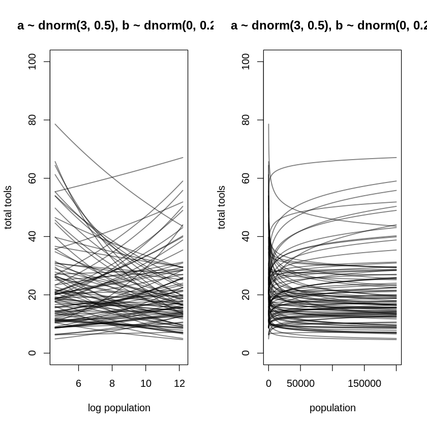
The right plot above shows the same diminishing returns on population discussed in the text, even though the curves now bend both ways. It’s unfortunate the author chose to introduce this concept of diminishing returns in the context of the Poisson model, as if there’s something special about it, e.g. that logging a predictor to a Poisson model is the only way to achieve diminishing returns. If you log a predictor in a plain old linear regression, you’ll achieve the same diminishing returns. That is, the influence of the predictor on the outcome will decrease as x increases, just as the instantaneous slope of the logarithm decreases as the argument increases in a graph of the logarithm.

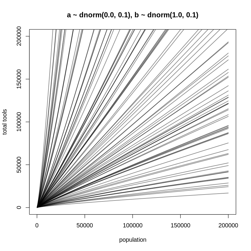
Introducing the idea of diminishing returns in the context of the Poisson distribution is also confusing because its link function is already a logarithm. In fact, why doesn’t the inverse link (exp) undo the log in a logged predictor? Consider the model again, assuming the predictor is logged:

\[\begin{split} \begin{align} y_i & = Poisson(\lambda) \\ log(\lambda) & = \alpha + \beta·log(x) \end{align} \end{split}\]

Applying the inverse link to \(\lambda\):

\[\begin{split} \begin{align} \lambda & = exp(\alpha + \beta·log(x)) \\ \lambda & = exp(\alpha) + exp(\beta·log(x)) \\ \lambda & = exp(\alpha) + exp(log(x^{\beta})) \\ \lambda & = exp(\alpha) + x^{\beta} \end{align} \end{split}\]

That is, this will only happen when \(\beta\) is inferred to about equal one. The following plot reproduces this situation. The code to produce this plot does not standardize x because doing so would scale the logarithmic axis (based on the natural logarithm) by the standard deviation of the data, making it harder to produce straight lines.

N <- 100
a <- rnorm(N, 0.0, 0.1)
b <- rnorm(N, 1.0, 0.1)
x_seq <- seq(from = log(100), to = log(200000), length.out = 100)
lambda <- sapply(x_seq, function(x) exp(a + b * x))
plot(NULL,
xlim = range(exp(x_seq)), ylim = c(0, 200000),
main='a ~ dnorm(0.0, 0.1), b ~ dnorm(1.0, 0.1)',
xlab = "population", ylab = "total tools"
)
for (i in 1:N) lines(exp(x_seq), lambda[i, ], col = grau(), lwd = 1.5)

11.4. Summary

It is important to never convert counts to proportions before analysis, because doing so destroys information about sample size.

The author indirectly touches at this through the UCBadmit example; the whole-school proportions don’t match the department-level proportions. He also indirectly touches at it in question 11H5. But he never really makes this point directly.

12.3. Ordered categorical outcomes

ERROR:

It is very common in the social sciences, and occasional [sic] in the natural sciences

12.3.2. Describing an ordered distribution with intercepts

The author switches between \(\alpha_k\) and \(\kappa_k\) for the log-cumulative-odds intercept (cutpoint) in this section. It looks like this is the result of a partial conversion to \(\kappa\) (for alliteration with cutpoint) rather than \(\alpha\).

12.3.3. Adding predictor variables

It would help to describe the log-cumulative-odds of each response k (\(\alpha_k\)) as a ‘cutpoint’ at the start of this section to help the reader get more intuition into why decreasing \(\alpha_k\) increases the expected mean count.

ERROR:

Finally loop over the first 50 samples in [sic] and plot their predictions

Finally loop over the first 50 samples in the posterior and plot their predictions

ERROR:

The trick here is to use pordlogit to compute the cumulative probability for each possible outcome value, from 1 to 7 [sic], using the samples

From 1 to 6; the author makes the same mistake a few sentences later.

ERROR:

In the upper-right [sic], action is now set to one.

Should be upper-middle; similar mistakes are made throughout this paragraph.

12.4. Ordered categorical predictors

Now the sum of every \(\delta_j\) is 1, and we can

The author has provided no constraint limiting the sum of the \(\delta_j\) to one at this point. In the code below he provides the constraint.

The beta is a distribution for two probabilities

Technically the Beta distribution is a distribution for one probability \(p\) and the Dirichlet distribution is for two or more probabilities. It’s likely the author is including the probability of not \(p\) (that is, \(q = 1 - p\)).

In the beta, these were the parameters α and β, the prior counts of success and failures, respectively.

The author used a different parameterization earlier in the text; see the Wikipedia page.

ERROR:

The easiest way to do this is the [sic] use pairs:

The easiest way to do this is to use pairs:

ERROR:

Is it is only Some College (SCol) that seems to have only

It is only Some College (SCol) that seems to have only

14.1.1. Simulate the population

ERROR:

And now in mathematical form:

These equations render correctly in the textbook (pdf) but not in VitalSource.

Note the set.seed(5) line above.

It’s not clear why the author is explaining set.seed at this point when readers will have seen it many times. Perhaps this section was part of other material and not reviewed.

14.1.3. The varying slopes model

and a vector of standard deviations sigma_cafe.

In the code, there is no clear way to specify the standard deviation among slopes and the standard deviation among intercepts separately. If you check precis you’ll see a vector, however.

14.3. Instruments and causal design

Of course sometimes it won’t be possible to close all of the non-causal paths or rule of (sic) unobserved confounds.

14.5. Continuous categories and the Gaussian process

14.5.1. Example: Spatial autocorrelation in Oceanic tools.

This will allow us to estimate varying intercepts for each society that account for non-independence in tools as a function of their geographical similarly.

This will allow us to estimate varying intercepts for each society that account for non-independence in tools as a function of their geographic distance.

In that model, the first part of the model is a familiar Poisson probably (sic) of the outcome variable.

The vertical axis here is just part of the total covariance function.

The author starts to use the term covariance function a lot, without explanation. See:

• Gaussian process

• Covariance function

First, note that the coefficient for log population, bp, is very much as it was before we added all this Gaussian process stuff.

Presumably the author means b rather than bp.

Second, those g parameters are the Gaussian process varying intercepts for each society.

Second, those k parameters are the Gaussian process varying intercepts for each society.

Like a and bp, they are on the log-count scale, so they are hard to interpret raw.

It’s true that k is on the log-count scale, but a is not.

14.5.2. Example: Phylogenetic distance.

Species, like islands, are more or less distance (sic) from one another.

15.1. Measurement error

15.1.2. Error on the outcome

Both the caption of Figure 15.2 and the text describing it expect a blue line and shading for the new regression (on the right figure). These do not exist.

15.2. Missing data

15.2.1. DAG ate my homework

the noisy (sic) level of the student’s house

15.2.2. Imputing primates

Do you think you can estimate the causal influence of M on \(R_B\)?

As long as we don’t include B* in the model, it looks like we could close all non-causal paths. We’d predict \(R_B\) with a binomial model.

because the locations of missing values have to (sic) respected

The model that imputes missing values, m15.3, has narrower

The author suddenly switches to models m15.3 and m15.4, which are from the section on dogs eating homework. Presumably the models were renamed at some point.

Both plots show imputed neocortex values in blue, with 89% compatibility intervals shown by

This is incorrect, the figure caption is correct.

15.3. Categorical errors and discrete absences

15.3.1. Discrete cats

Take a look at the posterior of m15.6 and verify that

The author almost surely meant m15.8

16.3. Ordinary differential nut cracking

The duration pf (sic) the bout in seconds

16.3.1. Scientific model

where k is a parameter that measures the rate of skill gain with age.

The paragraph before this one just said that we’re going to assume knowledge comes with age (and mass). The author meant to say this is a parameter that measures the rate of mass gain with age.

16.4.2. The statistical model

But if you are curious how to incorporate rounding into a statistical model, see the Overthinking box later on.

There is no Overthinking box on rounding error; in fact there are no more Overthinking boxes past this point.

The author uses \(\alpha_H\), \(\beta_H\), \(\alpha_L\), and \(\beta_L\) in the model under \(p_H\) and \(p_L\) but never defines them. These are new relative to the model in Predator-Prey Population Dynamics: the Lotka-Volterra model in Stan so it’s not surprising they were missed. If you check the code, we are using what the text called a “strong prior” for \(p\):

data(Lynx_Hare_model)
cat(Lynx_Hare_model)
flush.console()

# Taken from the `?dbeta` documentation
pl.beta <- function(a,b, asp = if(isLim) 1, ylim = if(isLim) c(0,1.1)) {
  if(isLim <- a == 0 || b == 0 || a == Inf || b == Inf) {
    eps <- 1e-10
    x <- c(0, eps, (1:7)/16, 1/2+c(-eps,0,eps), (9:15)/16, 1-eps, 1)
  } else {
    x <- seq(0, 1, length.out = 1025)
  }
  fx <- cbind(dbeta(x, a,b), pbeta(x, a,b), qbeta(x, a,b))
  f <- fx; f[fx == Inf] <- 1e100
  matplot(x, f, ylab="", type="l", ylim=ylim, asp=asp,
          main = sprintf("[dpq]beta(x, a=%g, b=%g)", a,b))
  abline(0,1,     col="gray", lty=3)
  abline(h = 0:1, col="gray", lty=3)
  legend("top", paste0(c("d","p","q"), "beta(x, a,b)"),
         col=1:3, lty=1:3, bty = "n")
  invisible(cbind(x, fx))
}

functions {
  real[] dpop_dt( real t,                 // time
                real[] pop_init,          // initial state {lynx, hares}
                real[] theta,             // parameters
                real[] x_r, int[] x_i) {  // unused
    real L = pop_init[1];
    real H = pop_init[2];
    real bh = theta[1];
    real mh = theta[2];
    real ml = theta[3];
    real bl = theta[4];
    // differential equations
    real dH_dt = (bh - mh * L) * H;
    real dL_dt = (bl * H - ml) * L;
    return { dL_dt , dH_dt };
  }
}
data {
  int<lower=0> N;              // number of measurement times
  real<lower=0> pelts[N,2];    // measured populations
}
transformed data{
  real times_measured[N-1];    // N-1 because first time is initial state
  for ( i in 2:N ) times_measured[i-1] = i;
}
parameters {
  real<lower=0> theta[4];      // { bh, mh, ml, bl }
  real<lower=0> pop_init[2];   // initial population state
  real<lower=0> sigma[2];      // measurement errors
  real<lower=0,upper=1> p[2];  // trap rate
}
transformed parameters {
  real pop[N, 2];
  pop[1,1] = pop_init[1];
  pop[1,2] = pop_init[2];
  pop[2:N,1:2] = integrate_ode_rk45(
    dpop_dt, pop_init, 0, times_measured, theta,
    rep_array(0.0, 0), rep_array(0, 0),
    1e-5, 1e-3, 5e2);
}
model {
  // priors
  theta[{1,3}] ~ normal( 1 , 0.5 );    // bh,ml
  theta[{2,4}] ~ normal( 0.05, 0.05 ); // mh,bl
  sigma ~ exponential( 1 );
  pop_init ~ lognormal( log(10) , 1 );
  p ~ beta(40,200);
  // observation model
  // connect latent population state to observed pelts
  for ( t in 1:N )
    for ( k in 1:2 )
      pelts[t,k] ~ lognormal( log(pop[t,k]*p[k]) , sigma[k] );
}
generated quantities {
  real pelts_pred[N,2];
  for ( t in 1:N )
    for ( k in 1:2 )
      pelts_pred[t,k] = lognormal_rng( log(pop[t,k]*p[k]) , sigma[k] );
}

Here’s a plot of that prior:

pl.beta(40, 200)

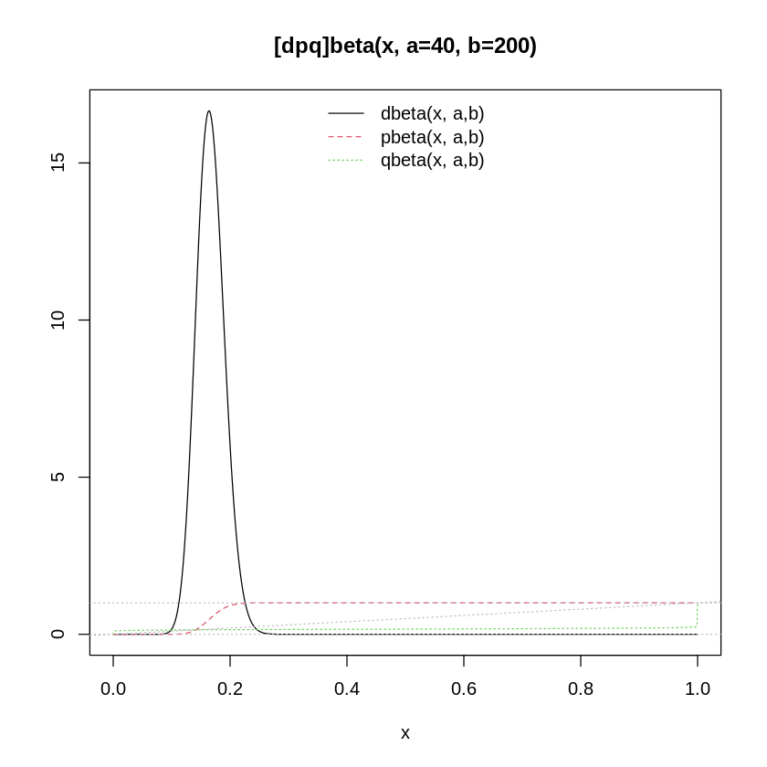
As discussed elsewhere, there are multiple beta distribution parameterizations. To confirm we are using the correct one, see:

• 20.1 Beta distribution | Stan Functions Reference

• Beta distribution - Wikipedia

16.4 Population dynamics

not that the distance (sic) past can influence the present.