
5.4 Graphical linear algebra#
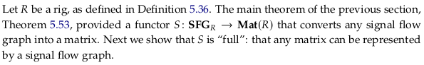
5.4.1 A presentation of Mat(R)#
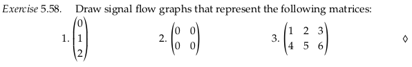
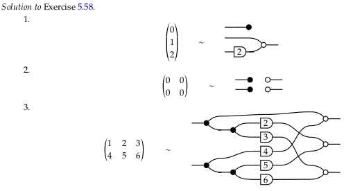
Exercise 5.58#

Reveal 7S answer
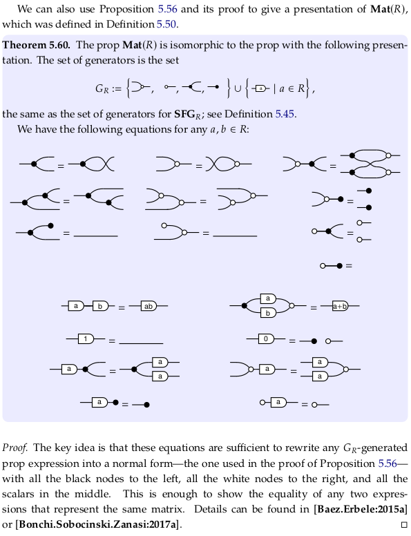
Exercise 5.59#
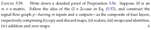
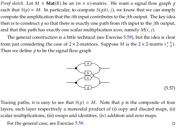
In stage (i) we’ll take the \(m\) inputs and make \(n\) copies of each to prepare for \(m*n\) scalar multiplications in stage (ii). In stage (iii) we’ll use swaps and identities to build a permutation matrix to convert the scaled data from a row-major to a column-major form. In the final stage (iv) we’ll use additions to sum across the now-contiguous column data.
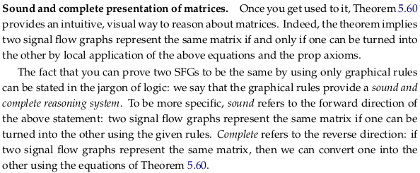
Theorem 5.60#
Sound and complete presentation of matrices.#
Two SFG can in general represent different matrices:
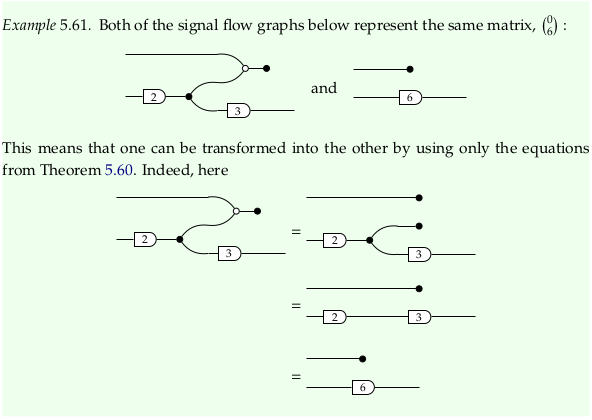
The sound property implies that if \(SFG_1\) can be converted into \(SFG_2\) using the given rules, then \(M_1\) and \(M_2\) are equal. The complete property implies that if \(M_1\) and \(M_2\) are equal, then \(SFG_1\) can be converted into \(SFG_2\) using the given rules. The second statement is clearly the Converse (logic) of the first. Example 5.61 is demonstrating an implication of the complete property. See also Completeness (logic) and Soundness.
Why use anything but the normal form to represent matrices? As Example 5.62 and 5.63 demonstrate, the non-normal form of a matrix can be much smaller (i.e. more efficient, with fewer additions and multiplications).
Example 5.61#
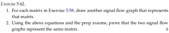
Exercise 5.62#

Reveal 7S answer
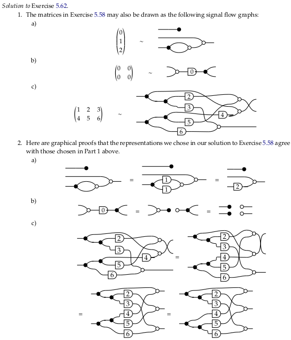
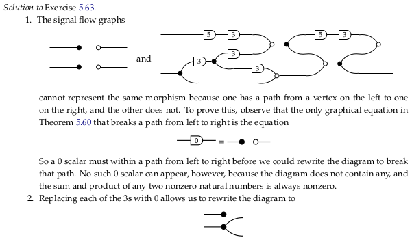
Exercise 5.63#
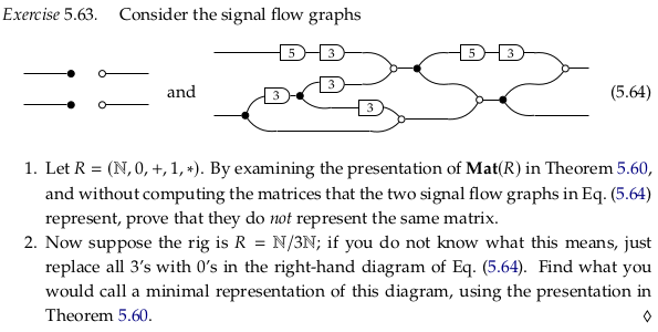
Consider part 1.. Calling the two inputs \(x_1\) and \(x_2\) (from top to bottom) and the two outputs \(y_1\) and \(y_2\), there’s clearly a non-zero contribution to \(y_1\) from \(x_1\). Following only the top wire, it’s at least \(5·3·5·3 = 225\) when the input is non-zero.
Note that because the semiring is the natural numbers, the inputs are always zero or greater.
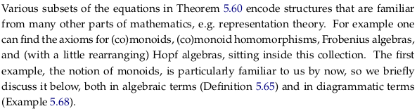
For part 2.:

Reveal 7S answer
5.4.2 Aside: monoid objects in a monoidal category#
Identity#
We often denote the identity morphism on a vertex v as either \(v\) or \(id_v\). Prefer the latter notation; otherwise this can be confusing because \(v\) can also mean the object \(v\), which is really a different thing. The articles Identity function and Category (mathematics) don’t introduce this same ambiguity (this ambiguity was explicitly introduced by the author in Section 3.2.1).
Prefer \(id_v\) to \(1_v\); the latter assumes the identity element is one (as in multiplication) although it is shorter.
There’s only ever one identity morphism on an object and it is both a left and right identity; see Identity element / Properties for a discussion of how the existence of both a left and right identity implies the two identities must be equal.
What does \(id\) mean, without any subscript, as in the upcoming Exercise 5.67? Often it means the Identity functor, which is not a morphism at all. Or is it? Do you assume that 0-morphisms don’t map structure, so 1-morphisms (functors) do? That’s thinking only in Set. Still, it may be more appropriate to write \(id_𝓒\) rather than \(id_C\) to make it clear this is a functor that can take as an argument any object in 𝓒 rather than the identity morphism on an object C. This isn’t to say that \(id_C\) couldn’t take an argument; in Set it would take elements of the set (an identity function).
This is closely related to the primordial ooze, that is, seeing functions/morphisms as “single” things/objects vs. seeing them as a collection of things/objects (a mapping defined for many objects). It’s likely this is the reason that sometimes we give id a subscript and sometimes we don’t; the former emphasizes that is one thing/object in some larger collection and the latter emphasizes that it is a collection of things itself (that could be subscripted/indexed as needed). Thinking in terms of both subscripts and arguments, the language of \(id_a(x)\) lets you essentially consider three levels at once. For more on subscripts vs applying arguments, see Indexed family.
Is \(id_{x_{x_x}}\) so bad? Clearly the subscripts are going to get so small as to be unreadable. The “solution” in many contexts seems to be to start with subscripts then move to argument application (see e.g. Operations with natural transformations) to get terms like \(id_{F(X)}\) (which would otherwise have been \(id(F(X))\) or \(id_{F_X}\)). For simplicity we’ll either follow this mixed pattern, or use all parentheses.
Can you “apply” a natural transformation the same way you apply an argument to a function or an object to a functor? See the first paragraph of Natural transformation, before all the nasty definitional details. The apparent difference is that a natural transformation typically takes a single functor F as an argument and produces a second functor G; it’s a transformation that is defined for only one input argument. Let’s simplify our thinking to identities, though, so we can more easily go up a level (“level shift” in the language of section 1.4.5). Who says there isn’t an identity function defined for all natural transformations? Call this id, so that \(id_\eta\) refers to the specific morphism we are talking about here.
We got where we wanted, but notice we’re using the language id (which we said before to prefer not to use, always including a subscript). We can only get away from this by seeing the “bigger picture” and making id just an example of morphism in a higher category. Try to do so yourself by mentally duplicating the following drawing below it, and introducing e.g. lowercase letters (a,b,c …) to assign names to the two objects in your new collection:

Even if you can draw the mental picture, it’s unlikely that you’ll need this level of abstraction. Adding abstraction creates complexity; if we had referred to id(η(G)) in the diagram above as plain old id, then we could have saved ourselves a lot of typing and referred to the identity function on id(η(G(1))) as simply id(1) (or \(id_1\)). This works as long as we don’t need to refer to the 1 in the context of id(η(F)) (our reference would then be ambiguous). In short, there’s a tradeoff between providing extra detail (potentially distracting, more work to provide) and potentially running into ambiguity.
Context creation#
All this likely hides the fact that when we “level shift” we are creating something new: a context. If we’re upshifting then we’re taking everything we know and trying to put it in a new box (seeing the big picture, seeing our currently focal object as part of a collection). If we’re downshifting then we’re creating a new box for something that we previously didn’t concern ourselves with (getting into the details, seeing our currently focal object as a collection that we need to open up and look through). Perhaps better terms are “upcreate” and “downcreate” to emphasize that these contexts don’t exist until we imagine them.
This gives Self-reference a whole new meaning. To avoid self-reference we have to define things that “just are” and we don’t question. This is referring to A as A rather than \(id_A\), which makes the world of A a real thing with e.g. multiple things inside it (a function). In the language of Strict 2-category these are the 0-cells: what we don’t question (at least for now). We don’t use negative numbers in this context; typically we’d reindex from 0 if we needed to add more details.
To “downcreate” is categorification. In fact the primary example of the concept given by the author and the article Categorification is seeing a natural number such as 5 as a set of objects of size five {apple, banana, cherry, dragonfruit, elephant}.
In computing this is related to dependencies. What objects do you “define” to simply exist? These become your dependencies in a particular domain. You don’t have to dig into your own definitions; you’ve taken them as axioms.
This is highly related to how a Monad (functional programming) creates a context for computation. When we’re programming and downcreating it’s easy to write a bunch of new code that only addresses what we care about: we get to decide the new bottom. When we’re upcreating this isn’t so easy. How do we share all that we know with higher levels? We often compress our results, even arguing that this is good. It’s in this context that it’s important to wire e.g. a Maybe monad dependency through all the layers.
If you could make the structure associated with a particular morphism part of the argument i.e. make it part of a set based on tuples, couldn’t you make sure it was preserved in any conversion? In that sense, it’s all data. What do you let be passed via context, and what must be passed on a case-by-case basis? Functional languages try to make it easy to pass information via context, so that it does get passed at all.
Contrast this with Identity (mathematics), which is actually an equality.
Define n⁰ (for non-negative n)#
The functor \(U\) in Exercise 5.69 sends \(n ∈ ℕ\) to the set \(ℝ^n\). What does this mean when n = 0? First, we should read \(ℝ^n\) as a Real coordinate space, not necessarily as a vector space (given the codomain of \(U\) is Set, but in general as well). See Real coordinate space § Examples; this defines \(ℝ^0\) as a singleton. Clearly this is the most popular/common definition in mathematics (the apparent consensus) per e.g. the hmakholm answer, but why is raising any number to the power of zero equal to one? Should numbers (or sets) to the power of zero equal one (or have cardinality one)?
Advantages#
See Empty product, with a variety of arguments for this convention.
If you want to reinterpret functions with \(n\) arguments as taking a member of \(ℝ^n\), then \(ℝ^0\) would correspond to constant functions. That is, functions that take zero arguments e.g. \(x = 7\). In this last example, is \(x\) a function/morphism from some “singleton” object (defining \(n^0 = 1\)), or is it an alias for 7 (defining \(n^0 = 0\))? Either way, we could write it \(x: ℝ^0 → ℝ^1 = 7\) (leaving \(ℝ^0\) ambiguous).
Said another way, must we define even constant objects as being with respect to something that already exists? This is highly related to the conversation about identity above.
If you take Dimension to mean the number of coordinates that are needed to specify the position of a point in context, then if your “context” is a point you need zero dimensions to specify your location.
Is this the equivalent to calling numpy.squeeze? In the case of numpy.squeeze, you have to supply dummy 0 arguments if you don’t remove the extra dimensions. If there are 2 or greater columns along one dimension of a relation, you can see it as being of order \(R^1\): you need to supply at least one argument to that context to supply which column you mean. If there is only one column, then you don’t really need to specify anything to that “context” (that dimension) to specify what data you mean. It’s up to you: feel free to squeeze or unsqueeze depending on your logical needs.
From this perspective, every dimension in a PyTorch tensor could “actually” be of zero or one dimension, despite the type reported by PyTorch. That is, the system could easily be holding onto no longer needed dimensions.
When you write a function from a singleton set to some other set e.g. f = x ↦ 2: {1} → {2,3} there’s really no need to supply the first argument. While f(1) is clearly going to be 2, you could have concluded the answer would be 2 without this argument. On the other hand, what would f(2) mean? It seems like it would be better to be explicit so you can catch apparent errors like this one. Per Initial and terminal objects, there can be multiple zero objects (even if they are unique up to unique isomorphism).
However, from the perspective of Free variables and bound variables, it doesn’t make sense to bind an argument if it doesn’t show up as a variable anywhere in the expression. To continue to provide the argument seems non-minimal. In the above, would you want an error if you supplied 1 rather than 0 to index a PyTorch tensor with a column of dimension 1? You could have prevented the error from even being possible by cleaning up your logic.
If you write this f(), are you applying the empty tuple ()? It seems so, see Function application. This “flat” horizontal stack is often a good visualization; the equivalent for a column vector is File:Real 0-space.svg, mentioned in Real coordinate space § Examples.
If you imagine \(5^3\) as a cube with 125 elements, then when you move to \(5^2\) you reduce one dimension to one. Similarly when you go from \(5^2\) to \(5^1\) (from a box to an array). To be consistent, you should define going from \(5^1\) to \(5^0\) as only collapsing the last dimension down to length one. This is similar to many other answers, such as The Count’s.
Many other answers argue for this approach merely because it’s convenient. See also:
https://math.stackexchange.com/questions/135 (all answers)
It’s convenient to use this definition to be able to use the trivial or zero vector space (see Examples of vector spaces). See also Dimension (vector space) and Zero-dimensional space.
Disadvantages#
If you see \(5^3\) as five groups of fives groups of five, then \(5^2\) as five groups of five, then \(5^1\) as a group of five, why wouldn’t \(5^0\) be zero groups, or zero? Perhaps the issue here is that “five” means “five elements” or “five groups of one” and so to remove the word “group” one more time would leave one.
It’s tempting to expect \(ℝ^0\) to be the empty set. If you see this as the set of tuples of size zero, then you may not want to count the empty tuple () as a tuple.
While the Vectornaut answer is somewhat convincing, why is “not doing anything” count as a mapping? If you had one bead and one paint, why wouldn’t there be two ways to paint the beads: assigning the one paint to the one bead, or doing nothing?
There’s no clear consensus on \(0^0\) and there may never be; see this MSE comment. Consider this table for the operation, which demonstrates some of the conflict:
Base/Exp |
0 |
1 |
2 |
|---|---|---|---|
0 |
? |
0 |
0 |
1 |
1 |
1 |
1 |
2 |
1 |
2 |
4 |
3 |
1 |
3 |
9 |
If we define a function (mathematics) as a total function, then the asymmetry in our definition leads to there always being one function out of the empty set but zero into it (see also Initial and terminal objects). That is, a function can’t be total and map to the empty set (if it has any elements in its source set). Is there a self-loop between the empty set and the empty set (i.e. \(0^0\))? Is it better to work with relations to avoid this issue? The empty function has always seemed strange.
You could see many of these corner cases as humans needing/wanting to define a function beyond where it currently has a semantic meaning. That is, functions are “total” by definition, and so unless you carefully define all your sets as being e.g. one element smaller then you may feel need like you need an answer for your function to remain total.
In different situations (with different semantics) different definitions may be appropriate. If you use only a definition that makes sense in most situations, then you may miss the opportunity to use a more appropriate definition to a situation (that allows for a much better or more elegant solution). When it comes to corner cases where multiple definitions may be acceptable, it gets hard to use Wikipedia (which only documents what are effectively common definitions).
Definition 5.65#
For a similar definition, see Monoid (category theory). The Wikipedia definition nearly exactly matches monoid in a monoidal category. Confusingly, in all definitions, both \(\mu\) and \(\eta\) are morphisms rather than natural transformations (despite being Greek letters).
The author glosses over the natural isomorphism \(\alpha\) in part (a) of his definition. He also apparently defines \(\eta\) as a function with signature \(0 → 1\) rather than \(1 → 1\) (allowable because \(I\) is a singleton set); without this assumption (b) doesn’t work.
The word “monoid” is being being thrown around a lot in this definition. First, there’s an almost-monoid associated with 𝓒 simply being a category based on the set (presumably a small category) of objects in 𝓒, the composition operator (∘ or ⨟), and all the identity morphisms. That is, one can view a small Category (mathematics) as similar to a monoid but without closure/totality properties (see also the row for “small category” in Template:Group-like structures). See also Groupoid. Still, a monoid is a small category but a small category is not a monoid (lacking totality/closure). This is worth mentioning because the standard composition operators provide one dimension where concatenation can happen on string diagrams, however. Because this isn’t a full monoid, you can’t concatenate just anything.
Arguably the composition direction is more like language/algebra (which is also not symmetric/commutative) and the monoidal direction is more like convolution/parallelism (or possible worlds).
This is distinct from the idea of a monoid being a small category with one object. For example, the monoid \((\{T,F\}, T, ∧)\) can be represented as a category with one object, two arrows, and the path equations \(TT = T, TF = F, FT = F, FF = F\). We can’t view it as monoid object unless we level shift to the category of sets, or the category of small categories.
Why must a monoid object only exist in a monoidal category? Because the identity for the monoid object \(\eta\) is (technically) dependent on the identity in the monoidal category \(I\), and the identity binary operation for the monoid object \(\mu\) is dependent on the monoidal category’s ⊗ to “concatenate” objects.
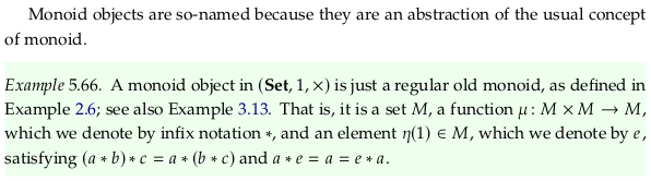
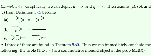
Example 5.66#
Exercise 5.67#
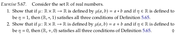
Let’s define \(id_ℝ: ℝ → ℝ\) specifically as \(id_ℝ(r) ↦ r\).
For 1. we have \(\mu: ℝ ⊗ ℝ → ℝ\) and \(id_ℝ: ℝ → ℝ\) so that \(\mu ⊗ id_ℝ: (ℝ ⊗ ℝ) ⊗ ℝ → ℝ ⊗ ℝ\).
Per the Cartesian product of functions this is specifically defined \((\mu ⊗ id_ℝ)((a,b), c) ↦ (a * b, c)\). Similarly:
Which are equal by associativity (the author ignores \(\alpha\) in his definition).
For part (b) we have \(\eta: 0 → 1 = 1\). So we have:
Example 5.68#
Exercise 5.69#
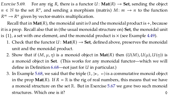
See also Monoidal functor and Monoidal natural transformation.
For 1., to show we preserve the monoidal unit:
To show we preserve the monoidal product:
which holds for all A and B in Mat(R), where + is the direct sum as given in Definition 5.50.
For 2. we can start by thinking of the specific monoids in Exercise 5.67. U(M) will be \(R^1\), so n = 1 in the prop Mat(R).
Wrap all the equations in Definition 5.65 in \(U\), and use all rules about preservation to reduce.
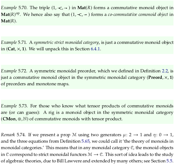
Other examples#
5.4.3 Signal flow graphs: feedback and more#
Exercise 5.77#
For part 1., the behavior of the addition icon is:
So the behavior of the reversed addition icon is:
For part 2., the behavior of the reversed copy icon is:
Combining directions.#
It’s not explicitly mentioned anywhere, so it’s worth calling out (before it’s needed) exactly what the zero-reverse and the discard-reverse mean. The original zero generator took nothing and produced zero; the original discard generator took anything and produced nothing. So the zero-reverse takes zero and produces nothing; the discard-reverse takes nothing and produces anything (it could be thought of as an “any” generator).
These definitions are perhaps confusingly written in terms of cause (or conversion), however, when a relation simply implies that certain tuples are valid.
One way to remember the icon for the zero signal (i.e. distinguish it from e.g. discard-reverse) is that the empty circle looks like a zero.
Consider the first diagram in this section in this light; the discussion of the “Compact closed structure” of \(\textbf{Rel}_R\) at the end of this section is also helpful. In short:
Definition 5.79#
Relative to Rel#
pip install -q xarray
How is this new \(\textbf{Rel}_R\) different than \(\textbf{Rel}\)? Clearly, there’s some relationship based on the name the author has decided to use here. It has more structure; while a morphism in \(\textbf{Rel}\) can be a subset of the product of any two sets (say A and B), the morphisms in \(\textbf{Rel}_R\) are constrained to be subsets of \(R^m × R^n\) (where R is the rig). This doesn’t imply the relation is no longer finite; consider the boolean matrices we encountered when discussing quantales (e.g. Example 2.102).
It does imply (at least conceptually) a rather inefficient storage format for matrices. Consider a 2×2 boolean matrix (an object in 𝔹²×𝔹² i.e. \(R^2 × R^2\) where the rig R = 𝔹). Taking 𝔹 = {0,1} we have 𝔹² = {00,01,10,11} so that this relation takes 4×4 = 16 bits to store. Consider the specific example of a boolean matrix taking 4 bits to store:
When we store (or think about) this as a relation, we have to consider every possible input (4 vectors of length 2) and provide a column of data for every possible output. For the example matrix above, applying the length-2 vector from the left:
import numpy as np
import xarray as xr

data = xr.DataArray(np.array(
    [
        [1,0,0,0],
        [0,0,1,0],
        [0,0,1,0],
        [0,0,1,0],
    ]),
    dims=("x", "y"), coords={"x": ["00", "01", "10", "11"], "y": ["00", "01", "10", "11"]}
)
data
Obviously these logical matrices will only get more sparse as we increase dimensionality. This is a clear example of decompression, taking a compact/efficent function/matrix and converting it to a complete list of examples. Since we’ve decompressed it, we may as well visualize the binary relation:

One could also see this as a list of pass/fail “unit” tests that we could write on the original function (the matrix). In this sense, the “behavioral” approach of section 5.4.3 is closer to machine learning models that define their model through large amounts of data.
Monoidal product in Rel#
What is the monoidal product in Rel? In Example 5.8, the monoidal product is apparently the disjoint union; the footnote almost states this directly. However, the article Category of relations states that the monoidal product (and the internal hom) are both the cartesian product (it also claims that the categorical product is the disjoint union). Now this definition is making the “product” of two sets is the monoidal product. Is the term “product” here referring to the Cartesian product or the categorical product (disjoint union)?
The issue is that while the categorical product in a category is quite tightly defined, the monoidal product is much more open to interpretation. That is, you can make a category monoidal in more than one way, i.e. there is no the monoidal product in Rel. We discussed in Chp. 2, for example, at least two monoidal structures on the Booleans and two on the real numbers. As discussed in FinVect, there are two common monoidal products on this category. For Set, see What other monoidal structures exist on the category of sets? - MO.
There’s no “right” monoidal product. As discussed in Why not use the Cartesian product for the monoidal category of modules? - MSE, we evaluate our structures based on how well they achieve our specific objectives. That doesn’t mean that we don’t explore widely-accepted structures on e.g. Wikipedia before inventing too many of our own, but it does imply we almost always need to be “creative” in the end. In the introduction to Chp. 3 this is put in terms of how there’s no best way to organize anything, such as your clothes.
The answer in Categorical product versus monoidal category - MSE directly states there can be more than one monoidal product. It also describes when the categorical product can be used as a monoidal product, and how (confusingly, if you’re using the term “categorical sum”) the categorical sum can serve as a monoidal product. It may be better to use the term “categorical product” alongside “coproduct” even if the two terms aren’t symmetric. See also Cartesian monoidal category.
All these comments beg the question: do both the Cartesian product and the categorical product (disjoint union) work to make Rel monoidal? Yes; the article Category of relations has been updated with a reference, and to avoid defining the monoidal structure on the category. The footnote on Example 5.8 unfortunately still defines the monoidal product as the disjoint union.
If you want more proof than a reference that defining the monoidal product as the Cartesian product forms a monoidal closed category, see Zhen’s answer in relations - Direct products in the category Rel - MSE. Using the variables of Product (category theory), the first half of the answer attempts to show that all the morphism pairs (\(f_1\), \(f_2\)) (referred to as \(\textbf{Rel}(X,Y) × \textbf{Rel}(X,Z)\)) are in one-to-one correspondence with functions f (referred to as \(\textbf{Rel}(X,Y⨿Z)\)). That is, it’s concerned with the OP’s question of what the direct/categorical product is in Rel.
In the second half of Zhen’s answer, he gets into the proof that Rel is monoidal closed with the cartesian product. The assertion that \(\textbf{Rel}(X, Y) = \mathscr{P}(X \otimes Y)\) is a consequence of the fact that every binary relation is a subset of the cartesian product of two sets. Therefore:
See the answer in Categorical product versus monoidal category - MSE for a less involved proof that defining the monoidal product to be the disjoint union of sets (categorical product) leads to a monoidal category; we simply need to observe that terminal objects exist in Rel (check Initial and terminal objects).
The answer to Does the product always exist in a monoidal category? - MSE is no, as indirectly covered by the fact that not all categories are a Cartesian monoidal category. The conversation also provides an example.
So what does the author mean when he says the “product of two sets” in this definition? If you web search that quote, all you’re going to get are references to the Cartesian product. If you take “product” to mean categorical product, however, then the author means the disjoint union.
Direct product and sum#
See Direct product and Direct sum. The former is apparently always a categorical product, but the latter is only usually (not always) a categorical coproduct (categorical sum). Still, it’s helpful to see that “direct” is almost a synonym for “categorical” (with a few exceptions).
Bookkeeping considerations#
Based on part (v) of the definition of a prop (the paragraph below Definition 5.2), given two morphisms m → n and p → q we expect the monoidal product on morphisms to have signature (m + p) → (n + q). Using some definitions from Exercise 5.80, this would imply B+C ⊆ \(R^{m+p} \times R^{n+q}\). Does this fit a monoidal product of either the disjoint union or the cartesian product?
If we were to use the disjoint union, then the domain of the new relation would be \(R^m ⊔ R^p\), and the codomain \(R^n ⊔ R^q\) (see previous commentary on Example 5.8). Let’s assume a finite rig \(R\), to avoid conversations about e.g. the cardinality of the continuum. Per Disjoint union, the cardinality of the disjoint union is the sum of the cardinalities of the terms, so the cardinality of \(R^m ⊔ R^p\) would be \(|R|^m + |R|^p\). If \(|R| = |𝔹| = m = p = 2\) as in the example above, then this is 8 rather than the expected 16.
The cartesian product would make B+C ⊆ \((R^m × R^n) × (R^p × R^q)\). Per Cartesian product, however, this operation is not associative. However, the cardinalities match since \(|R|^m|R|^n = |R|^{m+n}\) and it should not typically be difficult to establish an isomorphism between the two. In the example above with booleans, this would be \(((a,b),(c,d)) ↦ (a,b,c,d)\).
Exercise 5.80#
The product of the two sets B and C is then A = B × C or:
Notice that in both the answer to Exercise 5.77 and 5.80 the author doesn’t provide 2-tuple answers as this commentary has (corresponding to Binary relation). The advantage to the 2-tuple answers are they make the domain and codomain of the associated binary relation clear, and in particular distinct from its transpose. The advantage to the 3-tuple and 4-tuple answers (corresponding to Finitary relation) provided by the author is that they keep variables separate for a potential construction (via an isomorphism) of any binary relation.
Exercise 5.82#
The behavior of \(g\) is (copying Equation 5.75):
The behavior of \(h^{op}\) is (see Equation 5.76):
Per the discussion around Equation 5.78:
Exercise 5.83#
The behavior of \(g^{op}\) is (copying Equation 5.76):
The behavior of \(h\) is (see Equation 5.75):
Per the discussion around Equation 5.78:
Exercise 5.84#
Consider part 1.. See Kernel (linear algebra) and Kernel (category theory). Per table (5.52), the original zero generator had arity 0 → 1, taking nothing and producing a zero. As a behavior it’s:
The 0-reverse takes a zero and produces nothing, with arity 1 → 0. As a behavior it’s:
We can easily extend this definition to multiple dimensions (also changing the bound variable \(x\) to \(y\)):
Let’s use the result of Exercise 5.82 with \(h\) as above:
For part 2., see Cokernel and Linear map § Cokernel and Image (mathematics). Per table (5.52), the original discard generator had arity 1 → 0, taking anything and producing nothing. As a behavior it’s:
The discard-reverse takes nothing and produces anything, with arity 0 → 1. As a behavior it’s:
We can easily extend this definition to multiple dimensions:
Let’s take the result of Exercise 5.83 (with \(g\) replaced by \(d\), and \(h\) by \(g\), and \(p\) by \(n\)):
For part 3., see Linear subspace. Starting from the definition in (5.75):
We know that:
Exercise 5.85#
See Linear relation, distinct from e.g. Linear map and Linear function.
Let’s say we have two linear relations \(B_1\) and \(B_2\). Their composite is given by Equation (5.78):
Given \((x_1, z_1) \in B_1 ⨟ B_2\) and \((x_2, z_2) \in B_1 ⨟ B_2\) we show that \((x_1+x_2, z_1+z_2) \in B_1 ⨟ B_2\):
Given \(r \in R\) we show that \((rx, rz) \in B_1 ⨟ B_2\):
Compact closed structure.#
This section presents the snake equations for this category.