Practice: Chp. 6

source("iplot.R")
suppressPackageStartupMessages(library(rethinking))

6E1. List three mechanisms by which multiple regression can produce false inferences about causal effects.

Answer. Multicollinearity, Post-treatment bias, and Collider bias (the Chapter’s section titles).

6E3. List the four elemental confounds. Can you explain the conditional dependencies of each?

Answer. From the beginning of Section 6.4 (Confronting confounding):

• The Fork

• The Pipe

• The Collider

• The Descendant

For practice understanding which variables are ‘connected’ (dependent, covariate) without the help of automatic tools, see the DAGitty tutorial d-Separation Without Tears.

The Fork and Pipe actually have one and the same conditional dependency:

\[ X \perp \!\!\! \perp Y | Z \]

The Collider has no conditional dependencies, but \(X \perp Y\) unconditionally.

The Descendant is similar to the Collider. It still has \(X \perp Y\) unconditionally, but has the additional conditional dependencies:

\[\begin{split} \begin{align} X \perp \!\!\! \perp D | Z \\ Y \perp \!\!\! \perp D | Z \end{align} \end{split}\]

Notice X -> Z -> D and Y -> Z -> D are Pipes in themselves.

6E4. How is a biased sample like conditioning on a collider? Think of the example at the open of the chapter.

Answer. In a biased sample you’re presumably unaware of the additional variable; it’s simply not in your tables and generally not on your radar (e.g. in your causal diagram).

When you condition on a collider you are aware of the variable but instead choose to sample from the part of your table that is biased toward a particular realization of the variable.

source("practice-deconfound-chp6-models.R")

6M1. Modify the DAG on page 186 to include the variable V, an unobserved cause of C and Y: C ← V → Y. Reanalyze the DAG. How many paths connect X to Y? Which must be closed? Which variables should you condition on now?

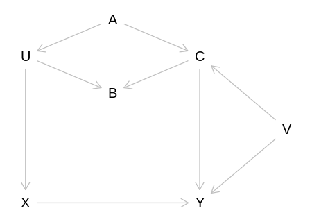
{ A }

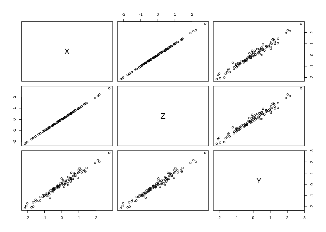
6M2. Sometimes, in order to avoid multicollinearity, people inspect pairwise correlations among predictors before including them in a model. This is a bad procedure, because what matters is the conditional association, not the association before the variables are included in the model. To highlight this, consider the DAG X → Z → Y. Simulate data from this DAG so that the correlation between X and Z is very large. Then include both in a model prediction Y. Do you observe any multicollinearity? Why or why not? What is different from the legs example in the chapter?

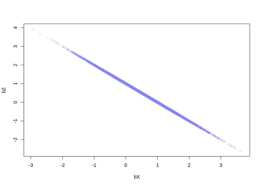
Answer. We still observe multicollinearity, most likely because it’s now impossible to distinguish the noise inherent in our measurement of Y from any noise added to Z relative to X. If the noise we add as part of generating Y is on the same scale as the noise added to Z, then we don’t observe this issue.

Removing predictors based on pairwise correlation is dangerous because we don’t know whether (in this case) either X or Z has a causal influence on Y. We really have no reason to prefer removing either X or Z from the analysis based on pairwise correlation, so we could easily remove the wrong one (X in this case) and infer that X has a direct (rather than total/indirect) causal influence on Y. If we were to then condition on Z, we’d be surprised with the results.

0.999773898191122

A precis: 4 × 4

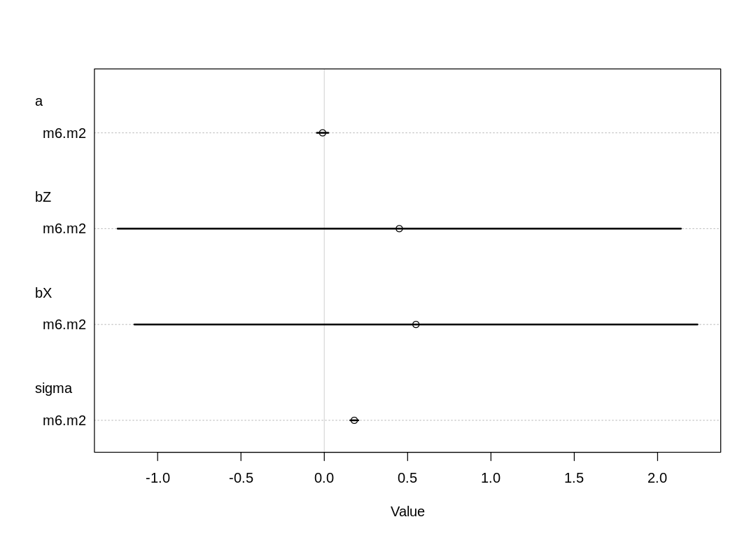
	mean	sd	5.5%	94.5%
	<dbl>	<dbl>	<dbl>	<dbl>
a	-0.00501325	0.01756539	-0.03308614	0.02305964
bZ	0.45105880	0.86229540	-0.92705579	1.82917339
bX	0.54829721	0.86204318	-0.82941429	1.92600871
sigma	0.17528736	0.01237711	0.15550634	0.19506837

6M3. Learning to analyze DAGs requires practice. For each of the four DAGs below, state which variables, if any, you must adjust for (condition on) to estimate the total causal influence of X on Y.

Answer. Reading the DAGs from the left to right, top to bottom:

1. Only Z, although A would not hurt (it is a competing exposure).

2. Only A. Conditioning on Z would measure direct effect rather than total effect.

3. None. Conditioning on Z would lead to collider bias.

4. Only A, which is otherwise a ‘Fork’ confounder (an ancestor of both X and Y).

See also:

• Terminology in Causal Diagrams: Covariate Roles

• Causal Intepretation of Multiple Regression: The Table 2 Fallacy

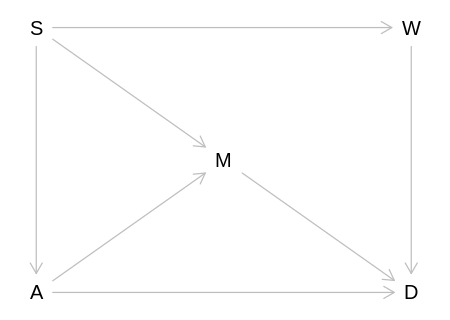
6H1. Use the Waffle House data, data(WaffleDivorce), to find the total causal influence of number of Waffle Houses on divorce rate. Justify your model or models with a causal graph.

Adjustment Sets:

{ A, M }
{ S }

6H2. Build a series of models to test the implied conditional independencies of the causal graph you used in the previous problem. If any of the tests fail, how do you think the graph needs to be amended? Does the graph need more or fewer arrows? Feel free to nominate variables that aren’t in the data.

A _||_ W | S
D _||_ S | A, M, W
M _||_ W | S

All three problems below are based on the same data. The data in data(foxes) are 116 foxes from 30 different urban groups in England. These foxes are like street gangs. Group size varies from 2 to 8 individuals. Each group maintains its own urban territory. Some territories are larger than others. The area variable encodes this information. Some territories also have more avgfood than others. We want to model the weight of each fox. For the problems below, assume the following DAG:

source('load-fox-models.R')
iplot(function() plot(dag_foxes), scale=10)
display_markdown("Implied Conditional Dependencies:")
display(impliedConditionalIndependencies(dag_foxes))

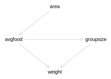
Implied Conditional Dependencies:

area _||_ grps | avgf
area _||_ wght | avgf

6H3. Use a model to infer the total causal influence of area on weight. Would increasing the area available to each fox make it heavier (healthier)? You might want to standardize the variables. Regardless, use prior predictive simulation to show that your model’s prior predictions stay within the possible outcome range.

Answer. We have nothing to condition on if we only care about the total causal effect of area on weight:

display(adjustmentSets(dag_foxes, exposure="area", effect="total"))

 {}

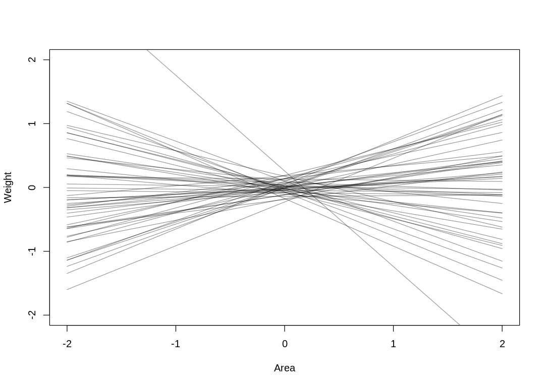
Answer. Assume the average area corresponds to the average weight in the priors (\(\beta_0\)):

prior <- extract.prior(mfox_Weight_Area)
mu <- link(mfox_Weight_Area, post=prior , data=list( Area=c(-2,2) ) )
iplot(function() {
    plot( NULL , ylab="Weight", xlab="Area", xlim=c(-2,2) , ylim=c(-2,2) )
    for ( i in 1:50 ) lines( c(-2,2) , mu[i,] , col=col.alpha("black",0.4) )
})

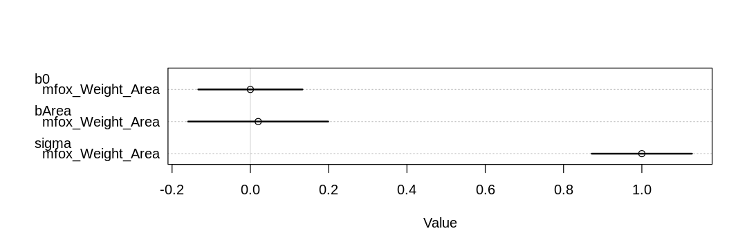
Presumably because a larger area implies both more food (increasing weight) and a larger group (decreasing weight, more mouths to feed) the total causal effect of area on weight is nearly zero:

iplot(function() plot(coeftab(mfox_Weight_Area)), ar=3)

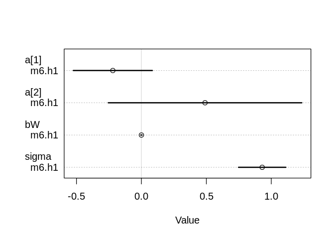
6H4. Now infer the causal impact of adding food to a territory. Would this make foxes heavier? Which covariates do you need to adjust for to estimate the total causal influence of food?”

Answer. We have nothing to condition on if we only care about the total causal effect of food on weight:

display(adjustmentSets(dag_foxes, exposure="avgfood", effect="total"))

 {}

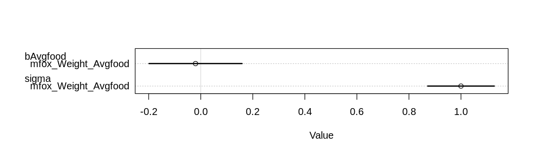
“Answer. Presumably because food also affects group size, and a larger group means more mouths to feed, there appars to be no noticeable impact of more food on weight:

iplot(function() plot(coeftab(mfox_Weight_Avgfood)), ar=3.5)

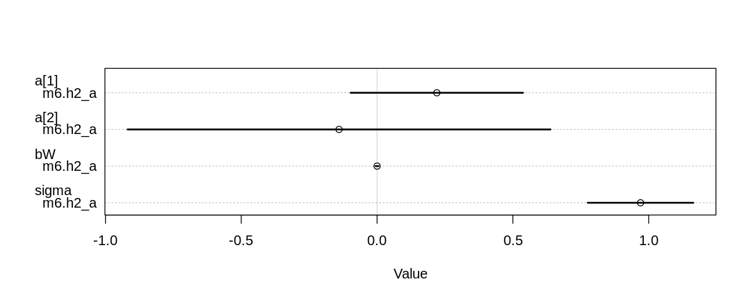
It’s more interesting to look at the direct affect of food on weight. To see this we’ll need to adjust for groupsize:

display(adjustmentSets(dag_foxes, exposure="avgfood", effect="direct"))

{ groupsize }

As expected, food has a positive influence on weight (bAvgfood is positive):

iplot(function() plot(coeftab(mfox_Weight_AvgfoodGroupsize)), ar=3)

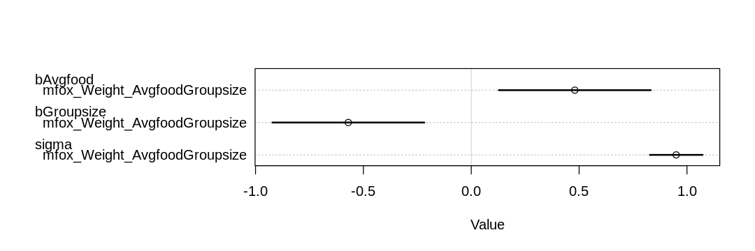
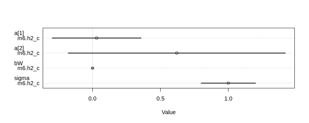
6H5. Now infer the causal impact of group size. Which covariates do you need to adjust for? Looking at the posterior distribution of the resulting model, what do you think explains these data? That is, can you explain the estimates for all three problems? How do they go together?

Answer. We need to adjust for only avgfood assuming we are interested in the total causal effect of groupsize (otherwise avgfood would be a confounder):

display(adjustmentSets(dag_foxes, exposure="groupsize", effect="total"))

{ avgfood }

See the model mfox_Weight_AvgfoodGroupsize above for a model that already includes only groupsize and avgfood. As expected, groupsize has a negative influence on weight (bGroupsize is negative) presumably because a bigger group means more mouths to feed.